rnalysis.filtering.CountFilter.split_clicom
- CountFilter.split_clicom(*parameter_dicts: dict, replicate_grouping: GroupedColumns | Literal['ungrouped'] = 'ungrouped', power_transform: bool | Tuple[bool, bool] = True, evidence_threshold: Fraction = 0.6666666666666666, cluster_unclustered_features: bool = False, min_cluster_size: PositiveInt = 15, plot_style: Literal['all', 'std_area', 'std_bar'] = 'all', split_plots: bool = False, parallel_backend: Literal['multiprocessing', 'loky', 'threading', 'sequential'] = 'loky', gui_mode: bool = False) Tuple[CountFilter, ...]
Clusters the features in the CountFilter object using the modified CLICOM ensemble clustering algorithm (Mimaroglu and Yagci 2012), and then splits those features into multiple non-overlapping CountFilter objects, based on the clustering result. The CLICOM algorithm incorporates the results of multiple clustering solutions, which can come from different clustering algorithms with differing clustering parameters, and uses these clustering solutions to create a combined clustering solution. Due to the nature of CLICOM, the number of clusters the data will be divided into is determined automatically. This modified version of the CLICOM algorithm can also classify features as noise, which does not belong in any discovered cluster.
- Parameters:
replicate_grouping (nested list of strings or 'ungrouped' (default='ungrouped')) – Allows you to group your data into replicates. Each replicate will be clustered separately, and used as its own clustering setup. This can minimize the influence of batch effects on the clustering results, and take advantage of repeated measures data to improve the accuracy of your clustering. If `replicate_grouping`=’ungrouped’, the data will be clustered normally as if no replicate data is available. To read more about the theory behind this, see the following publication: https://doi.org/10.1093/bib/bbs057
power_transform (True, False, or (True, False) (default=True)) – if True, RNAlysis will apply a power transform (Box-Cox) to the data prior to clustering. If both True and False are supplied, RNAlysis will run the initial clustering setups twice: once with a power transform, and once without.
evidence_threshold (float between 0 and 1 (default=2/3)) – determines whether each pair of features can be reliably clustered together. For example, if evidence_threshold=0.5, a pair of features is considered reliably clustered together if they were clustered together in at least 50% of the tested clustering solutions.
cluster_unclustered_features (bool (default=False)) – if True, RNAlysis will force every feature to be part of a cluster, even if they were not initially determined to reliably belong to any of the discovered clusters. Larger values will lead to fewer clusters, with more features classified as noise.
min_cluster_size (int (default=15)) – the minimum size of clusters the algorithm will seek. Larger values will lead to fewer clusters, with more features classified as noise.
parameter_dicts – multiple dictionaries, each corresponding to a clustering setup to be run. Each dictionary must contain a ‘method’ field with a clustering method supported by RNAlysis (‘k-means’, ‘k-medoids’, ‘hierarchical’, or ‘hdbscan’). The other fields of the dictionary should contain your preferred values for each of the clustering algorithm’s parameters. Yoy can specify a list of values for each of those parameters, and then RNAlysis will run the clustering algorithm with all legal combinations of parameters you specified. For example, {‘method’:’k-medoids’, ‘n_clusters’:[3,5], ‘metric’:[‘Euclidean’, ‘cosine’]} will run the K-Medoids algorithm four times with the following parameter combinations: (n_clusters=3,metric=’Euclidean’), (n_clusters=5, metric=’Euclidean’), (n_clusters=3, metric=’cosine’), (n_clusters=5, metric=’cosine’).
plot_style ('all', 'std_area', or 'std_bar' (default='all')) – determines the visual style of the cluster expression plot.
split_plots (bool (default=False)) – if True, each discovered cluster will be plotted on its own. Otherwise, all clusters will be plotted in the same Figure.
parallel_backend (Literal[PARALLEL_BACKENDS] (default='loky')) – Determines the babckend used to run the analysis. if parallel_backend not ‘sequential’, will calculate the statistical tests using parallel processing. In most cases parallel processing will lead to shorter computation time, but does not affect the results of the analysis otherwise.
- Returns:
returns a tuple of CountFilter objects, each corresponding to a discovered cluster.
- Examples:
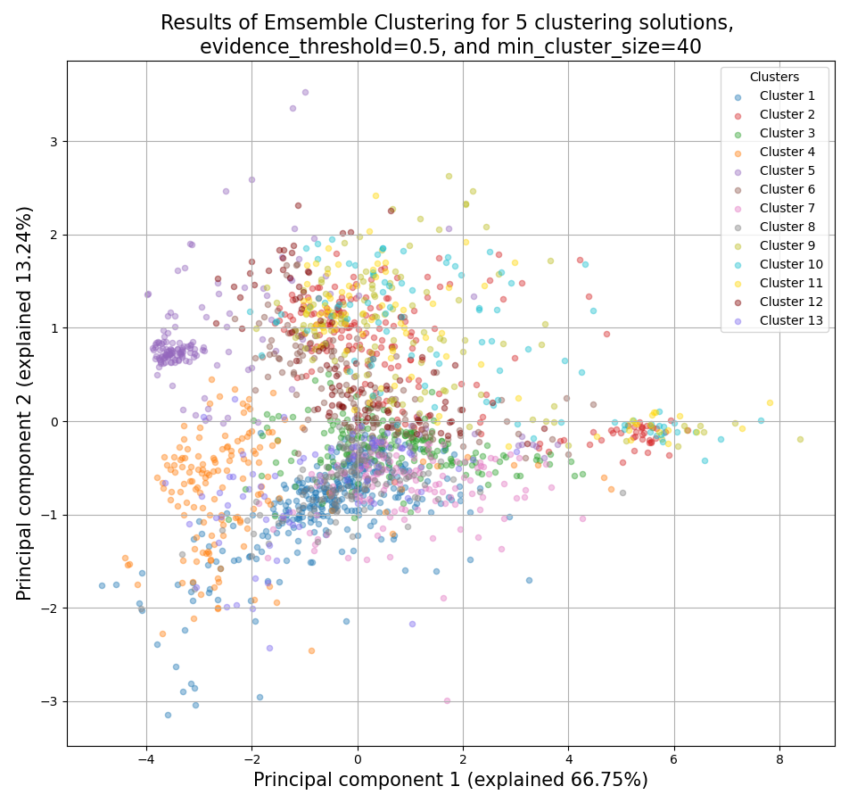
>>> from rnalysis import filtering
>>> dev_stages = filtering.CountFilter('tests/test_files/elegans_developmental_stages.tsv')
>>> dev_stages.filter_low_reads(100)
Filtered 44072 features, leaving 2326 of the original 46398 features. Filtered inplace.
>>> clusters = dev_stages.split_clicom(
... {'method': 'hdbscan', 'min_cluster_size': [50, 75, 140], 'metric': ['ys1', 'yr1', 'spearman']},
... {'method': 'hierarchical', 'n_clusters': [7, 12], 'metric': ['Euclidean', 'jackknife', 'yr1'],
... 'linkage': ['average', 'ward']}, {'method': 'kmedoids', 'n_clusters': [7, 16], 'metric': 'spearman'},
... power_transform=True, evidence_threshold=0.5, min_cluster_size=40)
Found 19 legal clustering setups.
Running clustering setups: 100%|██████████| 19/19 [00:12<00:00,  1.49 setup/s]
Generating cluster similarity matrix: 100%|██████████| [00:32<00:00, 651.06it/s]
Finding cliques: 100%|██████████| 42436/42436 [00:00<00:00, 61385.87it/s]
Done
Found 15 clusters of average size 153.60. Number of unclustered genes is 22, which are 0.95% of the genes.
Filtered 1864 features, leaving 462 of the original 2326 features. Filtering result saved to new object.
Filtered 2115 features, leaving 211 of the original 2326 features. Filtering result saved to new object.
Filtered 2122 features, leaving 204 of the original 2326 features. Filtering result saved to new object.
Filtered 2123 features, leaving 203 of the original 2326 features. Filtering result saved to new object.
Filtered 2128 features, leaving 198 of the original 2326 features. Filtering result saved to new object.
Filtered 2167 features, leaving 159 of the original 2326 features. Filtering result saved to new object.
Filtered 2179 features, leaving 147 of the original 2326 features. Filtering result saved to new object.
Filtered 2200 features, leaving 126 of the original 2326 features. Filtering result saved to new object.
Filtered 2204 features, leaving 122 of the original 2326 features. Filtering result saved to new object.
Filtered 2229 features, leaving 97 of the original 2326 features. Filtering result saved to new object.
Filtered 2234 features, leaving 92 of the original 2326 features. Filtering result saved to new object.
Filtered 2238 features, leaving 88 of the original 2326 features. Filtering result saved to new object.
Filtered 2241 features, leaving 85 of the original 2326 features. Filtering result saved to new object.
Filtered 2263 features, leaving 63 of the original 2326 features. Filtering result saved to new object.
Filtered 2279 features, leaving 47 of the original 2326 features. Filtering result saved to new object.
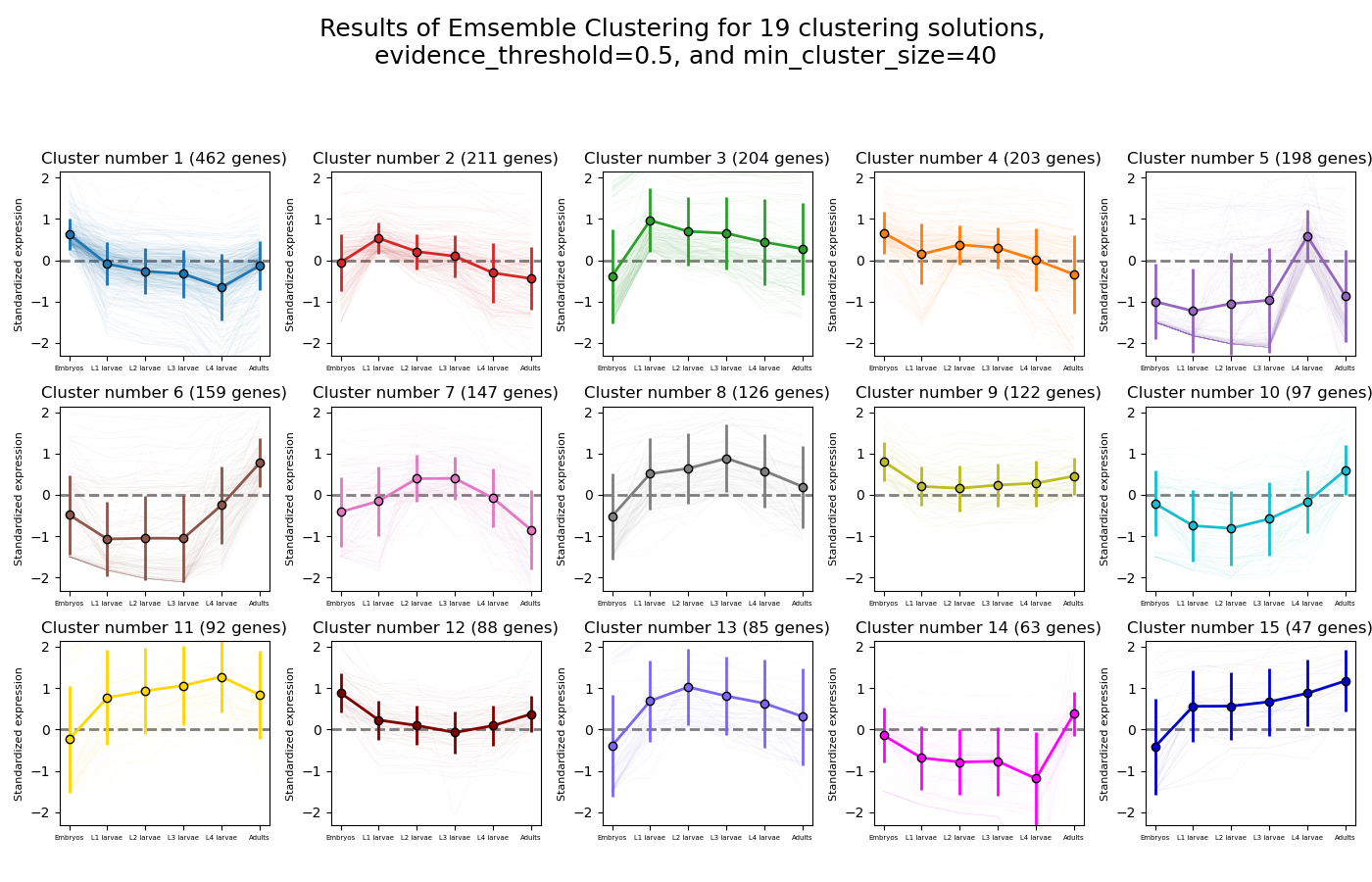
Example plot of split_clicom(plot_style=’all’)
Example plot of split_clicom()