The fastq module provides a unified programmatic interface to external tools that process FASTQ files.
Those currently include the CutAdapt adapter-trimming tool, the kallisto RNA-sequencing quantification tool,
the bowtie2 alignment tool, and the featureCounts feature counting tool.
The fastq module contains functions that interface with the different external tools.
Most of these tools require different sets of parameters for single-end vs paired-end reads, and therefore all of the functions in this module are split into single-end functions and paired-end functions.
We will start by importing the fastq module::
>>> from*RNAlysis*importfastq
You can now access the different functions of the fastq module, as explained in the sections below.
Cutadapt is a program that finds and removes adapter sequences, primers, poly-A tails and other types of unwanted sequencea from high-throughput sequencing reads.
Cutadapt can also trim bases based on their quality scores, high incidence of N (‘any’) bases, and perform basic filtering of reads.
This function takes two mandatory parameters:
* fastq_folder - the folder containing the FASTQ files you want to trim
* output_folder - the folder to which you want to write the trimmed FASTQ files
The other parameters allow you to specify the adapter/adapters you wish to trim according to their type (3’ adapters, 5’ adapters, or any position adapters), and to apply additional trimming/filtering actions.
You can read more about those parameters in the Cutadapt user guide.
This function takes three mandatory parameters:
* r1_files - list of paths the read#1 FASTQ files you want to trim
* r2_files - list of paths the read#2 FASTQ files you want to trim. The order of these should match the order of r1_files, so that they pair up.
* output_folder - the folder to which you want to write the trimmed FASTQ files
The other parameters allow you to specify the adapter/adapters you wish to trim according to their type (3’ adapters, 5’ adapters, or any position adapters), and to apply additional trimming/filtering actions.
Note that in paired-end mode, you can (and usually would) specify a different adapter for the read#1 files and the read#2 files.
You can read more about those parameters in the Cutadapt user guide.
kallisto is a program for quantifying abundances of transcripts from bulk and single-cell RNA sequencing data.
Kallisto uses an approach known as pseudoalignment - identifying the transcripts from which the reads could have originated, instead of trying to pinpoint exactly how the sequences of the reads and transcripts align.
This allows kallisto to run incredibly quickly, but still produce accurate and valid results.
You can read more about it in the kallisto publication.
To quantify expression using kallisto, in addition to processed FASTQ files, you will need a transcriptome indexed by kallisto, and a matching GTF file describing the names of the transcripts and genes in the transcriptome.
kallisto provides pre-indexed transcriptomes and their matching GTF files for most common model organisms, which can be downloaded here.
If your experiment requires a different transcriptome that is not available above, you can index any FASTA file through RNAlysis, by using the function kallisto_create_index:
The function takes one mandatory parameter - transcriptome_fasts. This should point to the path of a fasta file containing your target transcriptome.
Three additional optional paremeters are supported:
* kallisto_installation_folder - path to the installation folder of kallisto (or ‘auto’, if you have already added it to your PATH).
* kmer_length - length of the k-mer used to construct the index. Must be an odd integer <= 31. The default k-mer length is optimized for usual NGS read lengths (50-100bp) - if your reads are much shorter you may get better mapping results if you lower the k-mer length.
* make_unique - if True, replaces repeated target names with unique names.
Once you have an indexed transcriptome and trimmed FASTQ files, you can proceed with quantification.
If your FASTQ files contain single-end reads, you can use the kallisto_quantify_single_end function:
The function takes 5 mandatory parameters:
* fastq_folder - the folder containing the FASTQ files you want to quantify
* output_folder - the folder to which you want to write the output of the quantification
* index_file - path to your index file
* average_fragment_length - estimated average length of fragments produced by your library preperation protocol
* stdev_fragment_length - estimated standard deviation of the length of fragments produced by your library preperation protocol
The FASTQ files will be individually quantified and saved in the output folder, each in its own sub-folder.
Alongside these files, three .csv files will be saved: a per-transcript count estimate table,
a per-transcript TPM estimate table, and a per-gene scaled output table.
The per-gene scaled output table is generated using the scaledTPM method
(scaling the TPM estimates up to the library size) as described by
Soneson et al 2015 and used in the
tximport
R package. This table format is considered un-normalized for library size,
and can therefore be used directly by count-based statistical inference tools such as DESeq2.
RNAlysis will return this table once the analysis is finished.
If your FASTQ files contain paired-end reads (meaning, two FASTQ files for each sample - a ‘read#1’ file and ‘read#2’ file), you can quantify them using the kallisto_quantify_paired_end function::
The function takes 4 mandatory parameters:
* r1_files - list of paths the read#1 FASTQ files you want to quantify
* r2_files - list of paths the read#2 FASTQ files you want to quantify. The order of these should match the order of r1_files, so that they pair up.
* output_folder - the folder to which you want to write the output of the quantification
* index_file - path to your index file
The FASTQ file-pairs will be individually quantified and saved in the output folder, each in its own sub-folder.
Alongside these files, three .csv files will be saved: a per-transcript count estimate table,
a per-transcript TPM estimate table, and a per-gene scaled output table.
You can read more about these outputs in the section above.
To align reads using bowtie2, in addition to processed FASTQ files, you will need a reference genome indexed by bowtie2.
Bowtie2 provides pre-indexed genome files for most common model organisms.
These can be downloaded from the bowtie2 website (from menu on the right).
If your experiment requires a different transcriptome that is not available above, you can index any FASTA file (or files) through RNAlysis, by using the function bowtie2_create_index:
>>> genome='path/to/genome/file.fasta'# can also be a list of paths to FASTA files>>> output_folder='path/to/output/folder'>>> bowtie2_create_index(genome,output_folder)
This function takes two mandatory parameters:
* genome_fastas - path to FASTA file/files containing the reference sequences you wish to align to
* output_folder - the folder to which you want to write the genome index files
Once you have an index and trimmed FASTQ files, you can proceed with alignment.
If your FASTQ files contain single-end reads, you can align them using the bowtie2_align_single_end function:
>>> fastq_folder='path/to/fastq/files'>>> output_folder='path/to/output/folder'>>> index_file='path/to/index.1.bt2'# can be any of the index files>>> bowtie2_align_single_end(fastq_folder,output_folder,index_file)
The function takes 3 mandatory parameters:
* fastq_folder - the folder containing the FASTQ files you want to align
* output_folder - the folder to which you want to write the output of the alignment (SAM files)
* index_file - path to your index file. This can be either the path to one of the multiple index files bowtie2 generates (doesn’t matter which), or a path to the prefix/name of the index files. The important thing is that all of the index files are in the same folder.
Bowtie2 supports many additional paramaters - you can read about them in the bowtie2 manual.
Once you have an index and trimmed FASTQ files, you can proceed with alignment.
If your FASTQ files contain paired-end reads, you can align them using the bowtie2_align_paired_end function:
>>> read1_files=['path/to/sample1read1.fastq','path/to/sample2read1.fastq','path/to/sample3read1.fastq']>>> read2_files=['path/to/sample1read2.fastq','path/to/sample2read2.fastq','path/to/sample3read2.fastq']>>> output_folder='path/to/output/folder'>>> index_file='path/to/index.1.bt2'# can be any of the index files>>> bowtie2_align_paired_end(read1_files,read2_files,output_folder,index_file)
The function takes 4 mandatory parameters:
* r1_files - list of paths the read#1 FASTQ files you want to align
* r2_files - list of paths the read#2 FASTQ files you want to align. The order of these should match the order of r1_files, so that they pair up.
* output_folder - the folder to which you want to write the output of the alignment (SAM files)
* index_file - path to your index file. This can be either the path to one of the multiple index files bowtie2 generates (doesn’t matter which), or a path to the prefix/name of the index files. The important thing is that all of the index files are in the same folder.
Bowtie2 supports many additional paramaters - you can read about them in the bowtie2 manual.
featureCounts
is a highly efficient general-purpose read summarization program that counts mapped reads for genomic features such as genes, exons, promoter, gene bodies, genomic bins and chromosomal locations.
It can be used to count both RNA-seq and genomic DNA-seq reads.
featureCounts is part of the Subread package, which was also adapted into R as RSubread.
In order to use featureCounts through RNAlysis, you will need SAM/BAM files containing your aligned reads (such as those generated by bowtie2), and a GTF annotation file that matches the genome you aligned your reads to.
Furthermore, you will need to define the folder that contains your SAM/BAM files, and the folder to which you want to write the outputs:
Usually, you would want to assign reads to specific exons, and then sum up the exons into their corresponding genes, to get a final count of how many reads aligned to each gene.
If you want to count your reads differently, or your GTF file is non-standard, you can specify different values for the gtf_feature_type and gtf_attr_name parameters.
featureCounts supports many more options and parameters - you can read about them in the RNAlysis documentation and the featureCounts documentation.
While the mandatory paramters of this function are identical to those of single-end read counting, paired-end feature counting supports a few additional optional parameters.
Those include minimum/maximum fragment lengths, and the option to exclude chimeric reads or pairs where only one read was aligned.
The filtering module (rnalysis.filtering) is built to allow rapid and easy-to-understand filtering of various forms of RNA sequencing data. The module also contains specific methods for visualization and clustering of data.
The filtering module is built around Filter objects, which are containers for tabular sequencing data. You can use the different types of Filter objects to apply filtering operations to various types of tabular data. You will learn more about Filter objects in the next section.
All Filter objects (CountFilter, DESeqFilter, Filter, FoldChangeFilter) work on the same principles,
and share many of the same functions and features. Each of them also has specific filtering, analysis and visualisation functions. In this section we will look into the general usage of Filter objects.
In order to view a glimpse of the file we imported we can use the ‘head’ and ‘tail’ functions.
By default ‘head’ will show the first 5 rows of the file, and ‘tail’ will show the last 5 rows,
but you can specify a specific number of lines to show.
Now we can start filtering the entries in the file according to parameters of our choosing.
Various filtering operations are applied directly to the Filter object. Those operations do not affect the original csv file, but its representation within the Filter object.
For example, we can the function ‘filter_percentile’ to remove all rows that are above the specified percentile (in our example, 75% percentile) in the specified column (in our example, ‘log2FoldChange’):
>>> d.filter_percentile(0.75,'log2FoldChange')Filtered 7 features, leaving 21 of the original 28 features. Filtered inplace.
If we now look at the shape of d, we will see that 5954 rows have been filtered out of the object, and we remain with 17781 rows.
>>> d.shape(21, 6)
By default, filtering operations on Filter objects are performed in-place, meaning the original object is modified. However, we can save the results into a new Filter object and leave the current object unaffected by passing the argument ‘inplace=False’ to any filtering function within RNAlysis. For example:
>>> d=filtering.DESeqFilter("tests/test_files/test_deseq.csv")>>> d.shape(28, 6)>>> d_filtered=d.filter_percentile(0.75,'log2FoldChange',inplace=False)Filtered 7 features, leaving 21 of the original 28 features. Filtering result saved to new object.>>> d_filtered.shape(21, 6)>>> d.shape(28, 6)
In this case, the object ‘d’ remained unchanged, while ‘d_filtered’ became a new Filter object which contains our filtered results. We can continue applying filters sequentially to the same Filter object, or using ‘inplace=False’ to create a new object at any point.
Another useful option is to perform an opposite filter. When we specify the parameter ‘opposite=True’ to any filtering function within RNAlysis, the filtering function will be performed in opposite. This means that all of the genomic features that were supposed to be filtered out are kept in the object, and the genomic features that were supposed to be kept in the object are filtered out.
For example, if we now wanted to remove the rows which are below the 25% percentile in the ‘log2FoldChange’ column, we will use the following code:
>>> d.filter_percentile(0.25,'log2FoldChange',opposite=True)Filtered 7 features, leaving 21 of the original 28 features. Filtered inplace.
Calling this function without the ‘opposite’ parameter would have removed all values except the bottom 25% of the ‘log2FoldChange’ column. When specifying ‘opposite’, we instead throw out the bottom 25% of the ‘log2FoldChange’ column and keep the rest.
There are many different filtering functions within the filtering module. Some of them are subtype-specific (such as ‘filter_low_reads’ for CountFilter objects and ‘filter_significant’ for DESeqFilter objects), while others can be applied to any Filter object. You can read more about the different functions and their usage in the project’s documentation.
Performing set operations on multiple Filter objects
In addition to using regular filters, it is also possible to use set operations such as union, intersection, difference and symmetric difference to combine the results of multiple Filter objects. Those set operations can be applied to any Filter object, as well as to python sets. The objects don’t have to be of the same subtype - you can, for example, look at the union of a DESeqFilter object, an CountFilter object and a python set:
When performing set operations, the return type can be either a python set (default) or a string. This means you can use the output of the set operation as an input for yet another set operation. However, since the returned object is a set you cannot use Filter object functions such as ‘head’ and ‘save_csv’ on it, or apply filters to it directly. Intersection and Difference in particular can be used in-place, which applies the filtering to the first Filter object.
At any point we can save the current result of our filtering to a new csv file, by using the ‘save_csv’ function:
>>> d.save_csv()
If no filename is specified, the file is given a name automatically based on the filtering operations performed on it, their order and their parameters.
We can view the current automatic filename by looking at the ‘fname’ attribute:
>>> d.filter_percentile(0.75,'log2FoldChange')Filtered 7 features, leaving 21 of the original 28 features. Filtered inplace.>>> d.number_filters('baseMean','greater than',500)Filtered 6 features, leaving 15 of the original 21 features. Filtered inplace.>>> d.fname'D:/myfolder/test_deseq_below0.75baseMeangt500.csv'
Alternatively, you can specify a filename:
>>> d.save_csv('alternative_filename')
Instead of directly saving the results to a file, you can also get them as a set or string of genomic feature indices:
Sets of genomic feature indices can be used later for enrichment analysis using the enrichment module (see below).
Using an Attribute Reference Table for filter operations
An Attribute Reference Table contains various user-defined attributes (such as ‘genes expressed in intestine’, ‘epigenetic genes’ or ‘genes that have paralogs’) and their value for each genomic feature.
You can read more about the Attribute Reference Table format and loading an Attribute Reference Table in the Set and load a Reference Table section.
Using the function Filter.filter_by_attribute(), you can filter your genomic features by one of the user-defined attributes in the Reference Table:
>>> d=filtering.DESeqFilter("tests/test_files/test_deseq.csv")>>> d.filter_by_attribute('attribute1',ref='tests/test_files/attr_ref_table_for_examples.csv')Filtered 27 features, leaving 1 of the original 28 features. Filtered inplace.
Using a Biotype Reference Table for filter operations
A Biotype Reference Table contains annotations of the biotype of each genomic features (‘protein_coding’, ‘piRNAs’, ‘lincRNAs’, ‘pseudogenes’, etc).
You can read more about the Biotype Reference Table format and loading a Biotype Reference Table in the Set and load a Reference Table section.
Using the function Filter.filter_biotype_from_ref_table(), you can filter your genomic features by their annotated biotype in the Biotype Reference Table:
>>> d=filtering.DESeqFilter("tests/test_files/test_deseq.csv")>>> d.filter_biotype_from_ref_table('protein_coding',ref='tests/test_files/biotype_ref_table_for_tests.csv')Filtered 2 features, leaving 26 of the original 28 features. Filtered inplace.
You can also view the number of genomic features belonging to each biotype using the function Filter.biotypes_from_ref_table():
Filtering DESeq2 output files with filtering.DESeqFilter
DESeqFilter objects are built to easily filter differential expression tables, such as those returned by the R package DESeq2.
Like other Filter Objects, filtering operations on DESeqFilter are performed in-place by default, meaning the original object is modified.
Any csv file that contains differential expression analysis data with log2 fold change and adjusted p-values can be used as input for DESeqFilter.
By default, RNAlysis assumes that log2 fold change values will be specified under a ‘log2FoldChange’ column, and adjusted p-values will be specified under a ‘padj’ column (as is the default in differential expression tables generated by DESeq2):
baseMean
log2FoldChange
lfcSE
stat
pvalue
padj
WBGene00000021
2688.044
3.329404
0.158938
20.94783
1.96E-97
1.80E-94
WBGene00000022
365.813
6.101303
0.291484
20.93189
2.74E-97
2.40E-94
WBGene00000023
3168.567
3.906719
0.190439
20.51433
1.60E-93
1.34E-90
WBGene00000024
221.9257
4.801676
0.246313
19.49419
1.23E-84
9.82E-82
WBGene00000025
2236.186
2.477374
0.129606
19.11463
1.91E-81
1.46E-78
WBGene00000026
343.649
-4.03719
0.219781
-18.3691
2.32E-75
1.70E-72
WBGene00000027
175.1429
6.352044
0.347777
18.26471
1.58E-74
1.12E-71
WBGene00000028
219.1632
3.913657
0.217802
17.96885
3.42E-72
2.32E-69
Loading a file that follows this format into a DESeqFilter works similarly to other Filter objects:
If your differential expression table does not follow this format, you can specify the exact names of the columns in your table that contain log2 fold change values and adjusted p-values:
>>> d=filtering.DESeqFilter("tests/test_files/test_deseq.csv",log2fc_col='name of log2 fold change column',padj_col='name of adjusted p-value column')
Unique DESeqFilter functions (such as ‘filter_significant’ and ‘filter_abs_log2_fold_change’) will not execute properly if the log2 fold change column and adjusted p-value column are not defined correctly.
There are a few filtering operations unique to DESeqFilter. Those include ‘filter_significant’, which removes statistically-insignificant rows according to a specified threshold; ‘filter_abs_log2_fold_change’, removes rows whose absolute value log2 fold change is below the specified threshold; ‘filter_fold_change_direction’ which removes either up-regulated (positive log2 fold change) or down-regulated (negative log2 fold change) rows; and ‘split_fold_change_direction’ which returns a DESeqFilter object with only up-regulated features and a DESeqFilter object with only down-regulated features.
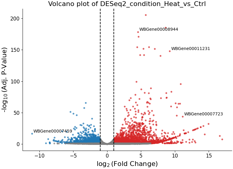
Data visualization and exploratory data analysis with DESeqFilter
DESeqFilter supports methods for visualization and exploratory analysis of differential expression data.
With DESeqFilter.volcano_plot, you can observe the direction, magnitude, and significance of differential expression within your data:
Filtering count matrices with filtering.CountFilter
CountFilter objects are capable of visualizing, filtering, normalizing, and clustering of read count matrices (the output of feature-counting software such as HTSeq-count and featureCounts).
Data can be imported into a CountFilter objects either from a csv file, or directly from HTSeq-count output files as explained below.
In principle, any csv file where the columns are different conditions/replicates and the rows include reads/normalized reads per genomic feature can be used as input for CountFilter. However, some CountFilter functions (such as ‘normalize_to_rpm_htseqcount’) will only work on HTSeq-count output files, and other unintended interactions may occur.
Generating an CountFilter object from a folder of HTSeq-count output .txt files
HTSeq-count receives as input an aligned SAM/BAM file. The native output of HTSeq-count is a text file with feature indices and read-per-genomic-feature, as well as information about reads that weren’t counted for any feature (alignment not unique, low alignment quality, ambiguous, unaligned, aligned to no feature).
An HTSeq-count output file would follow the following format:
WBGene00000001
376
WBGene00000002
1
WBGene00000003
1
WBGene00000004
18
WBGene00000005
1
WBGene00000006
3
WBGene00000007
6
WBGene00000008
0
WBGene00000009
1
WBGene00000010
177
__no_feature
32
__ambiguous
12
__too_low_aQual
1
__not_aligned
121
__alignment_not_unique
100
When running HTSeq-count on multiple SAM files (which could represent different conditions or replicates), the final output would be a directory of .txt files. RNAlysis can parse those .txt files into two csv tables: in the first each row is a genomic feature and each column is a condition or replicate (a single .txt file), and in the second each row represents a category of reads not mapped to genomic features (alignment not unique, low alignment quality, etc). This is done with the ‘from_folder_htseqcount’ function:
By deault, ‘from_folder_htseqcount’ does not save the generated tables as csv files. However, you can choose to save them by specifying ‘save_csv=True’, and specifying their filenames in the arguments ‘counted_fname’ and ‘uncounted_fname’:
It is also possible to automatically normalize the reads in the new CountFilter object to reads per million (RPM) using the unmapped reads data by specifying ‘norm_to_rpm=True’:
If you have previously generated a csv file from HTSeq-count output files using RNAlysis, or have done so manually, you can directly load this csv file into an CountFilter object as you would any other Filter object:
There are a few filtering operations unique to CountFilter. Those include ‘filter_low_reads’, which removes rows that have less than n reads in all columns.
CountFilter can normalize reads with either pre-made normalization methods RNAlysis supplies, or with user-defined scaling factors. Pre-normalized data can be used as input for CountFilter as well.
RNAlysis supplies the following normalization methods:
Relative Log Expression (RLE - ‘normalize_rle’), used by default by R’s DESeq2
Trimmed Mean of M-values (TMM - ‘normalize_tmm’), used by default by R’s edgeR
Quantile normalization, a generalization of Upper Quantile normalization (UQ - ‘normalize_quantile’), used by default by R’s Limma
Median of Ratios Normalization (MRN - ‘normalize_mrn’)
Reads Per Million (RPM - ‘normalize_to_rpm’)
To normalize a CountFilter with one of these functions, simply call the function with your preferred parameters, if there are any. For example:
The resulting CountFilter object will be normalized with the scaling factors (dividing the value of each column by the value of the corresponding scaling factor).
To normalize a CountFilter that originated from HTSeq-count to reads per million, we need a csv table with the special counters that appear in HTSeq-count output:
The resulting CountFilter object will be normalized to RPM with the formula (1,000,000 * reads in cell) / (sum of aligned reads + __no_feature + __ambiguous + __alignment_no_unique)
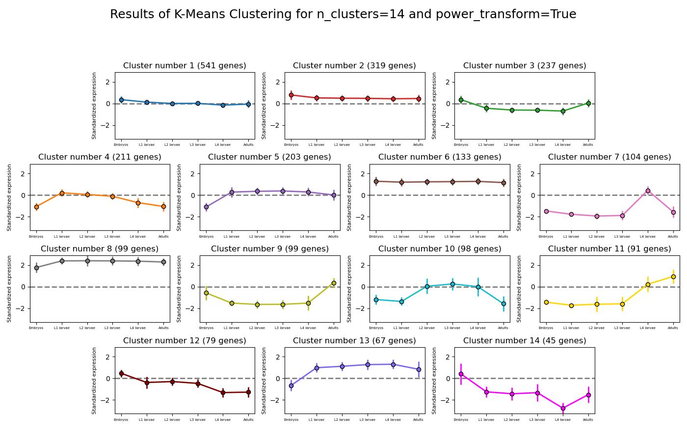
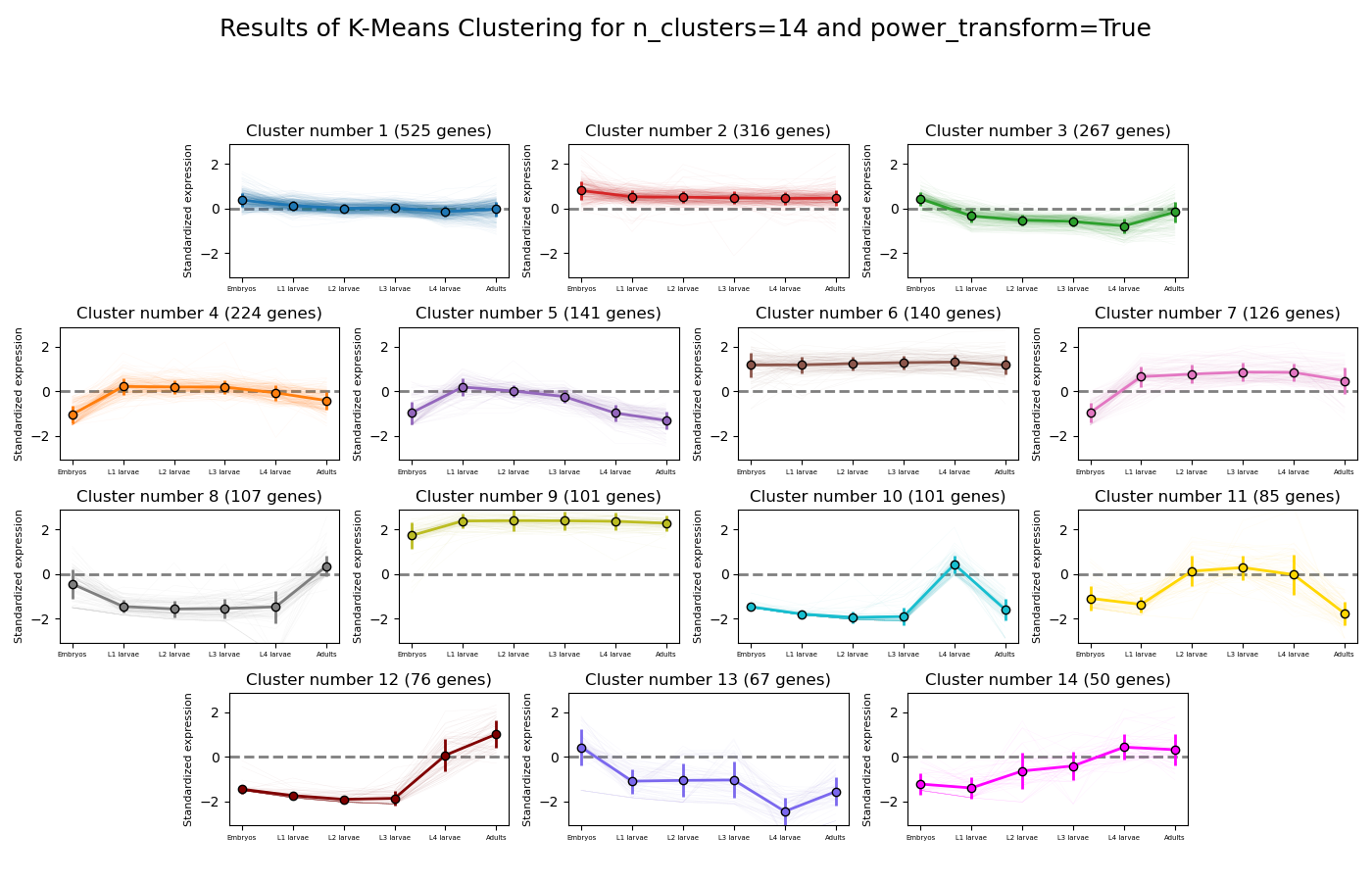
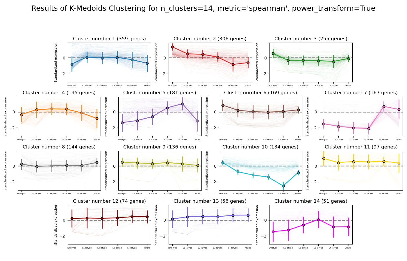
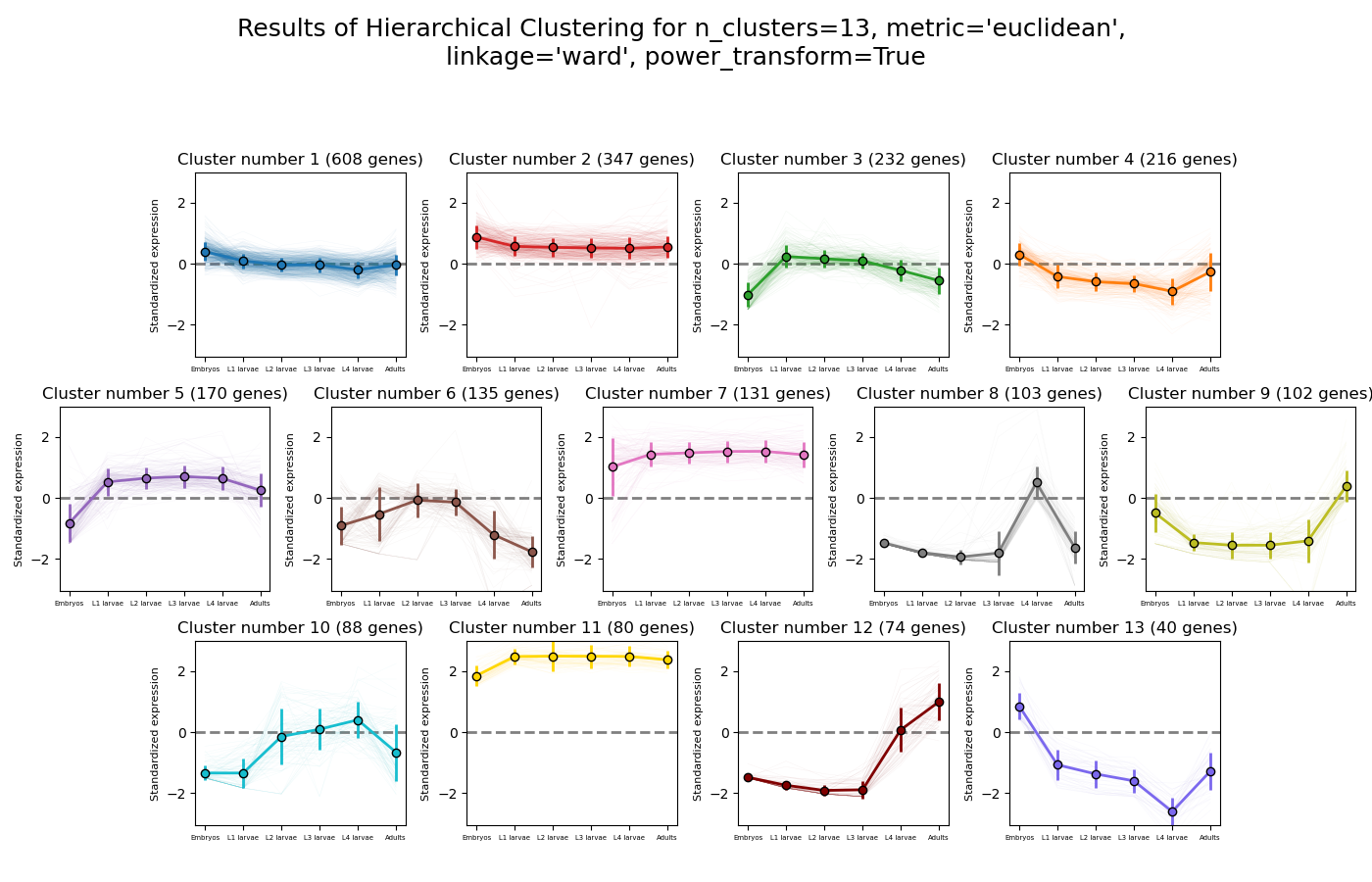
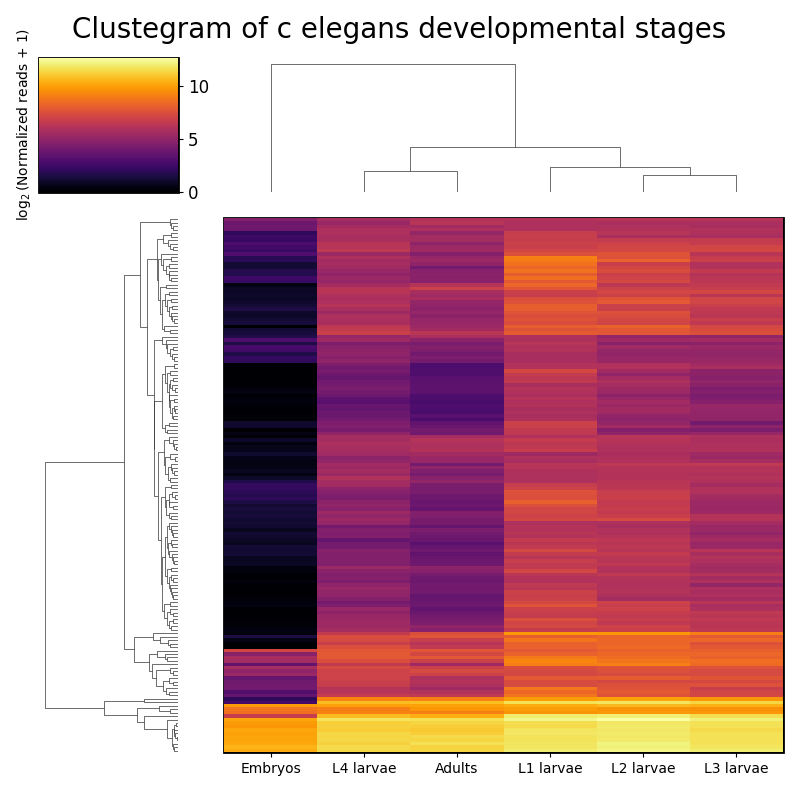
RNAlysis supports a wide variety of clustering methods, which can group genomic features into clusters according to their similarity across different samples.
When clustering genomic features in a CountFilter object, the called function returns a tuple of CountFilter objects, with each object corresponding to one cluster of genomic features.
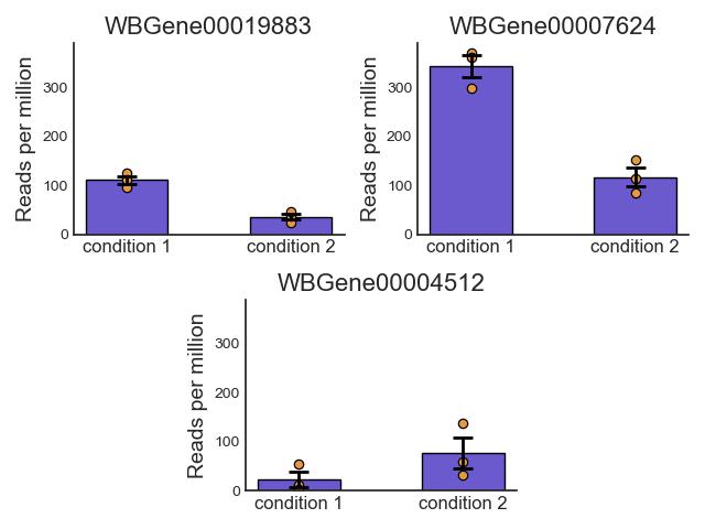
Expression plots of the resulting clusters can be generated in one of multiple styles:
Example expression plot of clustering results with plot_style=’all’
Example expression plot of clustering results with plot_style=’std_area’
Example expression plot of clustering results with plot_style=’std_bar’
The expression plots can also by split into separate graphs, one for each discovered cluster.
All clustering methods in RNAlysis which require you to specify the expected number of clusters (such as K in K-Means clustering) allow multiple ways of specifying the number of clusters you want to find.
You can specify a single value:
>>> counts=CountFilter("tests/test_files/counted.csv")>>> five_clusters=counts.split_kmeans(n_clusters=5)Filtered 20 features, leaving 2 of the original 22 features. Filtering result saved to new object.Filtered 7 features, leaving 15 of the original 22 features. Filtering result saved to new object.Filtered 20 features, leaving 2 of the original 22 features. Filtering result saved to new object.Filtered 20 features, leaving 2 of the original 22 features. Filtering result saved to new object.Filtered 21 features, leaving 1 of the original 22 features. Filtering result saved to new object.>>> print(len(five_clusters))5
You can specify a list of values to be used, and each value will be calculated and returned separately:
>>> counts=CountFilter("tests/test_files/counted.csv")>>> five_clusters,two_clusters=counts.split_kmeans(n_clusters=[5,2])Filtered 21 features, leaving 1 of the original 22 features. Filtering result saved to new object.Filtered 20 features, leaving 2 of the original 22 features. Filtering result saved to new object.Filtered 20 features, leaving 2 of the original 22 features. Filtering result saved to new object.Filtered 20 features, leaving 2 of the original 22 features. Filtering result saved to new object.Filtered 7 features, leaving 15 of the original 22 features. Filtering result saved to new object.Filtered 4 features, leaving 18 of the original 22 features. Filtering result saved to new object.Filtered 18 features, leaving 4 of the original 22 features. Filtering result saved to new object.>>> print(len(five_clusters))5>>> print(len(two_clusters))2
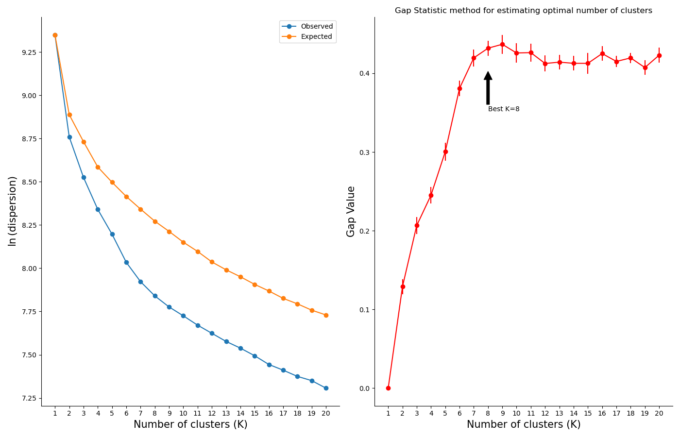
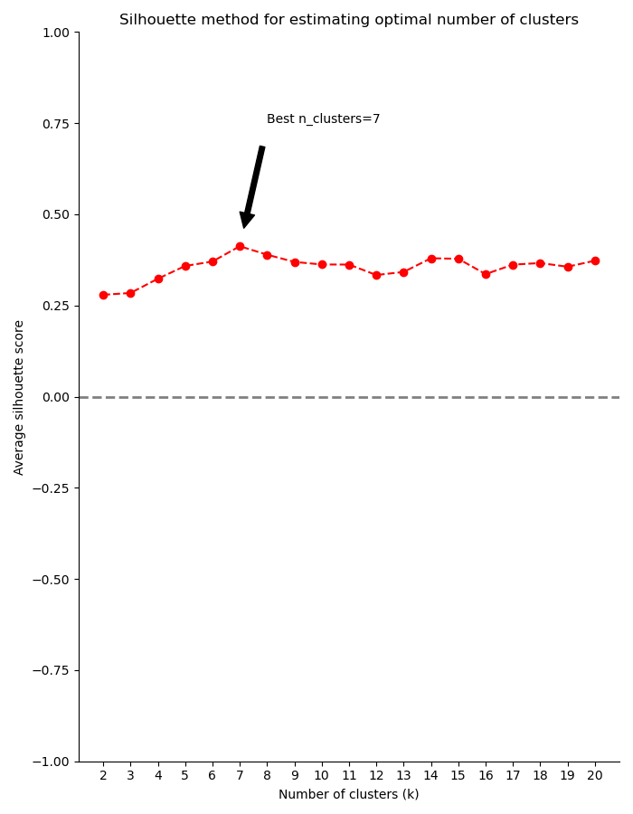
Finally, you can use a model selection method to estimate the number of clusters in your dataset. RNAlysis supports both the Silhouette method and the Gap Statistic method:
>>> counts=CountFilter("tests/test_files/counted.csv")>>> silhouette_clusters=counts.split_kmeans(n_clusters='silhouette')Estimating the optimal number of clusters using the Silhouette method in range 2:5...Using the Silhouette method, 4 was chosen as the best number of clusters (k).Filtered 20 features, leaving 2 of the original 22 features. Filtering result saved to new object.Filtered 6 features, leaving 16 of the original 22 features. Filtering result saved to new object.Filtered 20 features, leaving 2 of the original 22 features. Filtering result saved to new object.Filtered 20 features, leaving 2 of the original 22 features. Filtering result saved to new object.>>> print(len(silhouette_clusters))4>>> gap_stat_clusters=counts.split_kmeans(n_clusters='gap')Estimating the optimal number of clusters using the Gap Statistic method in range 2:5...Using the Gap Statistic method, 2 was chosen as the best number of clusters (K).Filtered 4 features, leaving 18 of the original 22 features. Filtering result saved to new object.Filtered 18 features, leaving 4 of the original 22 features. Filtering result saved to new object.>>> print(len(gap_stat_clusters))2
To help in evaluating the result of these model selection methods, RNAlysis will also plot a summary of their outcome:
K-means is a clustering method which partitions all of the data points into K clusters by minimizing the squared eucliean distance between points within each cluster.
The algorithm is initiated by picking a random starting point, and therefore the exact clustering results can change between runs.
The main advantage of K-means clustering is its simplicity - it contains one main tuning parameter (K, the expected number of clusters in the data).
The K-medoids method is very similar to K-means. The main difference between the two is the way they define clusters and the distances between them:
K-medoids picks one data point as the ‘center’ (medoid) of each cluster.
In addition, K-medoids attempts to minimize the sum of dissimilarities within each cluster, instead of minimizing squared euclidean distance.
Due to these differences, the K-medoids algorithm supports the use of distance metrics other than eucliean distance through the metric parameter.
K-medoids clustering in RNAlysis supports the following distance metrics:
Hierarchical clustering (or agglomerative clustering) is clustering method which aims to build a hierarchy of clusters.
In agglomerative hierarchical clustering, each data points starts in its own clusters.
The clustering algorithm then uses a distance metric (a measure of distance between pairs of data points)
and a linkage criterion
(determines the distance between sets of data points as a function of the pairwise distances between observations)
to group merge data points into clusters, and then further group those clusters into larger clusters based on their similarity.
Eventually, all of the observations are connected into a hierarchical tree.
We can decide to ‘cut’ the tree at any height in order to generate the final clustering solution.
This can be done by either specifying the estimated number of clusters like in K-means,
or by specifiying a distance threshold above which clusters will not be merged.
Hierarchical clustering in RNAlysis supports the following distance metrics:
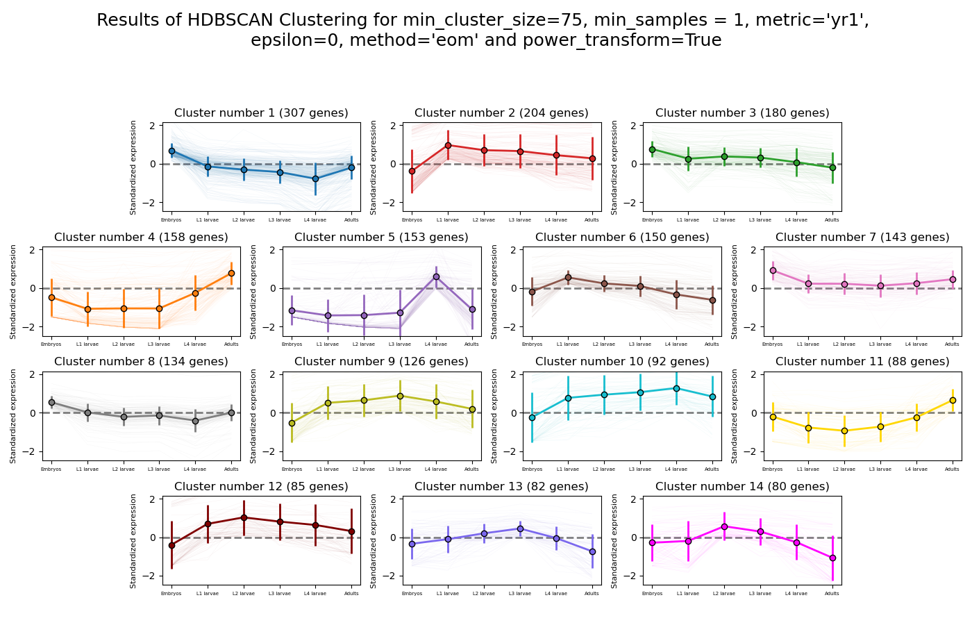
HSBSCAN makes relatively few assumptions about the data - it assumes that the data contains noise, as well as some real clusters which we hope to discover.
Unlike most other clustering methods, HDBSCAN does not force every data point to belong to a cluster. Instead, it can classify data points as outliers, excluding them from the final clustering solution.
HDBSCAN does not require you to guess the number of clusters in the data. The main tuning parameter in HDBSCAN is minimum cluster size (min_cluster_size), which determines the smallest “interesting” cluster size we expect to find in the data.
HDBSCAN supports additional tuning parameters, which you can read more about in the HDBSCAN documentation:
HDBSCAN in RNAlysis supports the following distance metrics:
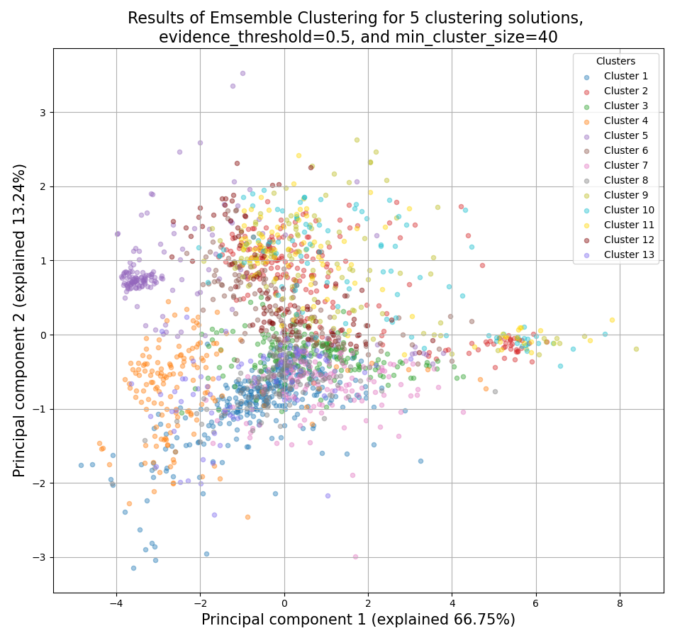
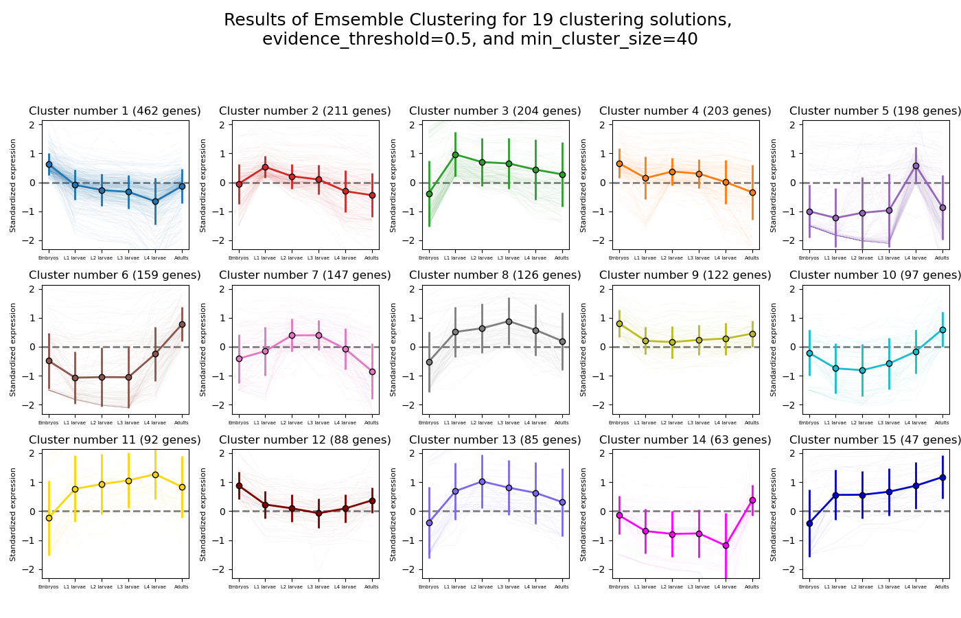
CLICOM is an ensemble-based clustering algorithm (see https://doi.org/10.1016/j.eswa.2011.08.059 ).
The CLICOM algorithm incorporates the results of multiple clustering solutions, which can come from different clustering algorithms with differing clustering parameters, and uses these clustering solutions to create a combined clustering solution.
CLICOM offers multiple advantages over more traditional clustering methods:
The ensemble clustering approach allows you to combine the results of multiple clustering algorithms with multiple tuning parameters, potentially making up for the weaknesses of each individual clustering method, and only taking into account patterns that robustly appear in many clustering solutions.
Unlike most other clustering methods, CLICOM does not have to force every data point to belong to a cluster. Instead, it can classify data points as outliers, excluding them from the final clustering solution.
CLICOM does not require you to guess the final number of clusters in the data. The main tuning parameter in HDBSCAN is the evidence threshold (evidence_threshold).
RNAlysis offers a modified implementation of CLICOM. This implementation of CLICOM supports a few tuning parameters, in addition to the clustering solutions themselves:
Moreover, ths modified version of the algorithm can cluster each batch of biological/technical replicates in your data separately, which can reduce the influence of batch effect on clustering results, and increases the accuracy and robustness of your clustering results.
evidence_threshold: a higher evidence threshold leads to fewer, large clusters, with fewer features being classified as outliers.
cluster_unclustered_features: if True, CLICOM will force every feature to belong to a discovered cluster. Otherwise, features can be classified as noise and remain unclustered.
min_cluster_size: determines the minimal size of a cluster you would consider meaningful. Clusters smaller than this would be classified as noise and filtered out of the final result, or merged into other clusters (depending on the value of cluster_unclustered_features).
replicates_grouping: allows you to group samples into technical/biological batches. The algorithm will then cluster each batch of samples separately, and use the CLICOM algorithm to find an ensemble clustering result from all of the separate clustering results.
In addition to the commonly-used distance metrics, such as euclidean distance and spearman correlation, RNAlysis offers a selection of distance metrics that were either developed especially for transcriptomics clustering, or found to work particularly well for transcriptomics clustering.
Those methods include:
1. jackknife distance - a modified Pearson dissimilarity coefficient.
Instead of measuring the linear correlation between expression levels of two genes, you measure the linear correlation coefficient N times (where N is the number of samples in the data), every time excluding a single sample from the correlation, and then taking the smallest correlation coefficient found.
The correlation score is then converted into a dissimilarity score.
This distance metric can detect linear correlation, like Pearson correlation, but is less sensitive to extreme values.
(see Heyer, Kruglyak and Yooseph 1999).
2. YR1 distance - a distance metric developed especially for time-series gene expression data.
This distance metric combines the Pearson dissimilarity, along with the positon of the minimal and maximal values of each sample, and the agreement of their slopes. These three values are combined into a single distance score.
This means that the YR1 metric captures more accurately the shape of the expression pattern of each gene, and ranks genes with similar expression patterns as more similar to one another.
(see Son and Baek 2007).
3. YS1 distance - a distance metric developed especially for time-series gene expression data.
This distance metric combines the Spearman dissimilarity, along with the positon of the minimal and maximal values of each sample, and the agreement of their slopes. These three values are combined into a single distance score.
This means that the YS1 metric captures more accurately the shape of the expression pattern of each gene, and ranks genes with similar expression patterns as more similar to one another.
(see Son and Baek 2007).
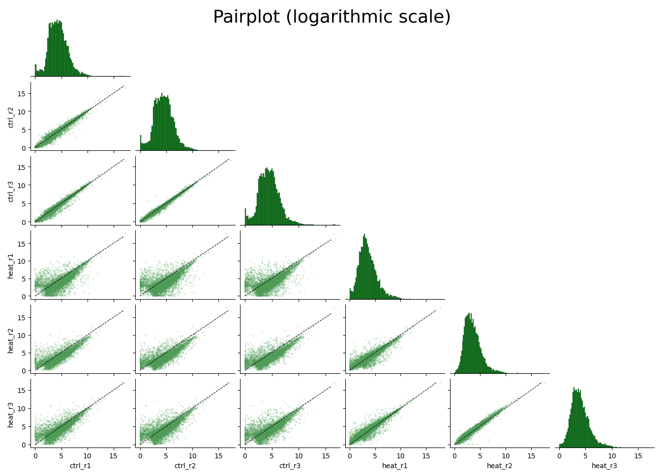
Data visualization and exploratory data analysis with CountFilter
CountFilter includes multiple methods for visualization and exploratory analysis of count data.
With CountFilter.pairplot, you can get a quick overview of the distribution of counts within each sample, and the correlation between different samples:
by default, FoldChangeFilter assumes that fold change is calculated as (numerator_reads+1)/(denominator_reads+1), and does not support 0 and inf values. If you load a csv file which contains 0 and/or inf values into a FoldChangeFilter object, unintended results and interactions may occur.
Unlike other Filter object, the underlying data structure storing the values is a pandas Series and not a pandas DataFrame, and lacks the Columns attribute.
Like with other objects from the Filter family, you can simply load a pre-existing or pre-calculated csv file into a FoldChangeFilter object. However, in addition to the file path you will also have to enter the name of the numerator condition and the name of the denominator condition:
>>> f=filtering.FoldChangeFilter('tests/test_files/fc_1.csv','name of numerator condition','name of denominator condition')
The names of the conditions are saved in the object attributes ‘numerator’ and ‘denominator’:
>>> f.numerator'name of numerator condition'>>> f.denominator'name of denominator condition'
Warning
by default, FoldChangeFilter assumes that fold change is calculated as (mean_numerator_reads+1)/(mean_denominator_reads+1), and does not support 0 and inf values. If you load a csv file which contains 0 and/or inf values into a FoldChangeFilter object, unintended results and interactions may occur.
Generating fold change data from an existing CountFilter object
We will now calculate the fold change between the mean of condition1 and condition2. Fold change is calculated as (mean_numerator_reads+1)/(mean_denominator_reads+1). We will need to specify the numerator columns, the denominator columns, and the names of the numerator and denominator. Specifying names is optional - if no names are specified, they will be generator automatically from columns used as numerator and denominator. Since we have multiple replicates of each condition, we will specify all of them in a list:
In this example we did not specify names for the numerator and denominator, and therefore they were generated automatically:
>>> f.numerator"Mean of ['cond1_rep1', 'cond1_rep2']">>> f.denominator"Mean of ['cond2_rep1', 'cond2_rep2']"
We now have a FoldChangeFilter object that we can perform further filtering operations on.
Performing randomization tests on a FoldChangeFilter object
You can perform a randomization test to examine whether the fold change of a group of specific genomic features (for example, genes with a specific biological function) is significantly different than the fold change of a background set of genomic features.
To perform a randomization test you need two FoldChangeFilter objects: one which contains the fold change values of all background genes, and another which contains the fold change values of your specific group of interest. For example:
>>> f=filtering.FoldChangeFilter('tests/test_files/fc_1.csv','numerator','denominator')>>> f_background=f.filter_biotype_from_ref_table('protein_coding',ref='tests/test_files/biotype_ref_table_for_tests.csv',inplace=False)#keep only protein-coding genes as referenceFiltered 9 features, leaving 13 of the original 22 features. Filtering result saved to new object.>>> f_test=f_background.filter_by_attribute('attribute1',ref='tests/test_files/attr_ref_table_for_examples.csv',inplace=False)Filtered 6 features, leaving 7 of the original 13 features. Filtering result saved to new object.>>> rand_test_res=f_test.randomization_test(f_background)Calculating... group size observed fold change ... pval significant0 7 2.806873 ... 0.360264 False[1 rows x 5 columns]
The output table would look like this:
group size
observed fold change
expected fold change
pval
significant
7
2.806873
2.51828
0.36026
False
Sequentially applying filtering operations using Pipelines
Pipeline objects allow you to group together multiple operations from the filtering module (such as filtering, splitting, normalizing, plotting or describing your data), and apply this group of operations to Filter objects of your choice in a specific and consistent order.
Pipelines make your workflow easier to read and understand, help you avoid repetitive code, and makes your analyses more reproducible and less error-prone.
Because every Filter object has its own unique functions, a particular Pipeline can only contain functions of a specific Filter object type, and can only be applied to objects of that type.
By default, a new Pipeline’s filter_type is Filter, and can only contain general functions from the filtering module that can apply to any Filter object.
If we wanted, for example, to create a Pipeline for DESeqFilter objects, we would have to specify the parameter filter_type:
One we have an empty Pipeline, we can start adding functions to it.
We can do that either via the function’s name:
>>> from*RNAlysis*importfiltering>>> pipe=filtering.Pipeline('DESeqFilter')>>> pipe.add_function('filter_significant')Added function 'DESeqFilter.filter_significant()' to the pipeline.
or via the function itself:
>>> from*RNAlysis*importfiltering>>> pipe=filtering.Pipeline('DESeqFilter')>>> pipe.add_function(filtering.DESeqFilter.filter_significant)Added function 'DESeqFilter.filter_significant()' to the pipeline.
We can also specify the function’s arguments. We can specify both non-keyworded and keyworded arguments, just as we would if we called the function normally:
>>> from*RNAlysis*importfiltering>>> pipe=filtering.Pipeline()>>> pipe.add_function(filtering.Filter.filter_biotype_from_ref_table,biotype='protein_coding')Added function 'Filter.filter_biotype_from_ref_table(biotype='protein_coding')' to the pipeline.>>> pipe.add_function('number_filters','column1','gt',value=5,opposite=True)Added function 'Filter.number_filters('column1', 'gt', value=5, opposite=True)' to the pipeline.
We can also view the functions currently in the Pipeline object, their arguments, and their order:
Just like with other functions in the filtering module, the functions in a Pipeline can be applied either inplace or returned as a new object.
You can determine that via the inplace argument of the function Pipeline.apply_to():
>>> from*RNAlysis*importfiltering>>> # create the pipeline>>> pipe=filtering.Pipeline('DESeqFilter')>>> pipe.add_function(filtering.DESeqFilter.filter_missing_values)Added function 'DESeqFilter.filter_missing_values()' to the pipeline.>>> pipe.add_function(filtering.DESeqFilter.filter_top_n,by='padj',n=3)Added function 'DESeqFilter.filter_top_n(by='padj', n=3)' to the pipeline.>>> pipe.add_function('sort',by='baseMean')Added function 'DESeqFilter.sort(by='baseMean')' to the pipeline.>>> # load the Filter object>>> d=filtering.DESeqFilter('tests/test_files/test_files/test_deseq_with_nan.csv')>>> # apply the Pipeline not-inplace>>> d_filtered=pipe.apply_to(d,inplace=False)Filtered 3 features, leaving 25 of the original 28 features. Filtering result saved to new object.Filtered 22 features, leaving 3 of the original 25 features. Filtering result saved to new object.Sorted 3 features. Sorting result saved to a new object.>>> # apply the Pipeline inplace>>> pipe.apply_to(d)Filtered 3 features, leaving 25 of the original 28 features. Filtered inplace.Filtered 22 features, leaving 3 of the original 25 features. Filtered inplace.Sorted 3 features. Sorted inplace.
Note that only functions that can be applied inplace (such as filtering/normalizing) will be applied inplace.
If our pipeline contained other types of functions, they will not be applied inplace, and will instead be returned at the end of the Pipeline.
If we apply a Pipeline with functions that return additional outputs (such as Figures, DataFrames, etc), they will be returned in a dictionary alongside the Filter object:
>>> from*RNAlysis*importfiltering>>> # create the pipeline>>> pipe=filtering.Pipeline('DESeqFilter')>>> pipe.add_function('biotypes_from_ref_table',ref='tests/test_files/test_files/biotype_ref_table_for_tests.csv')Added function 'DESeqFilter.biotypes_from_ref_table(ref='tests/test_files/test_files/biotype_ref_table_for_tests.csv')' to the pipeline.>>> pipe.add_function('filter_biotype_from_ref_table','protein_coding',ref='tests/test_files/test_files/biotype_ref_table_for_tests.csv')Added function 'DESeqFilter.filter_biotype_from_ref_table('protein_coding', ref='tests/test_files/test_files/biotype_ref_table_for_tests.csv')' to the pipeline.>>> pipe.add_function('biotypes_from_ref_table',ref='tests/test_files/test_files/biotype_ref_table_for_tests.csv')Added function 'DESeqFilter.biotypes_from_ref_table(ref='tests/test_files/test_files/biotype_ref_table_for_tests.csv')' to the pipeline.>>> # load the Filter object>>> d=filtering.DESeqFilter('tests/test_files/test_files/test_deseq_with_nan.csv')>>> # apply the Pipeline not-inplace>>> d_filtered,output_dict=pipe.apply_to(d,inplace=False)Biotype Reference Table used: tests/test_files/test_files/biotype_ref_table_for_tests.csvBiotype Reference Table used: tests/test_files/test_files/biotype_ref_table_for_tests.csvFiltered 2 features, leaving 26 of the original 28 features. Filtering result saved to new object.Biotype Reference Table used: tests/test_files/test_files/biotype_ref_table_for_tests.csv>>> print(output_dict['biotypes_1']) genebiotypeprotein_coding 26pseudogene 1unknown 1>>> print(output_dict['biotypes_2']) genebiotypeprotein_coding 26>>> # apply the Pipeline inplace>>> output_dict_inplace=pipe.apply_to(d)Biotype Reference Table used: tests/test_files/test_files/biotype_ref_table_for_tests.csvBiotype Reference Table used: tests/test_files/test_files/biotype_ref_table_for_tests.csvFiltered 2 features, leaving 26 of the original 28 features. Filtered inplace.Biotype Reference Table used: tests/test_files/test_files/biotype_ref_table_for_tests.csv
When an output dictionary is returned, the keys in the dictionary will be the name of the function appended to the number of call made to this function in the Pipeline (in the example above, the first call to ‘biotypes_from_ref_table’ is under the key ‘biotypes_1’, and the second call to ‘biotypes_from_ref_table’ is under the key ‘biotypes_2’); and the values in the dictionary will be the returned values from those functions.
We can apply the same Pipeline to as many Filter objects as we want, as long as the type of the Filter object matches the Pipeline’s filter_type.
If you have previously exported a Pipeline, or you want to use a Pipeline that someone else exported, you can import Pipeline files into any RNAlysis session.
RNAlysis Pipelines are saved as YAML (.yaml) files. Those files contain the name of the Pipeline, the functions and parameters added to it, as well as some metadata such as the time it was exported.
To import a Pipeline into RNAlysis, use the Pipeline.import_pipeline() method.
RNAlysis’s enrichment module (rnalysis.enrichment) can be used to perform various enrichment analyses including Gene Ontology (GO) enrichment and enrichment for user-defined attributes. The module also includes basic set operations (union, intersection, difference, symmetric difference) between different sets of genomic features.
The enrichment module is built around FeatureSet objects. A Featureset is a container for a set of gene/genomic feature IDs, and the set’s name (for example, ‘genes that are upregulated under hyperosmotic conditions’). All further anslyses of the set of features is done through the FeatureSet object.
A FeatureSet object can now be initialized by one of three methods.
The first method is to specify an existing Filter object:
>>> my_filter_obj=filtering.CountFilter('tests/test_files/counted.csv')# create a Filter object>>> my_set=enrichment.FeatureSet(my_filter_obj,'a name for my set')
The second method is to directly specify a python set of genomic feature indices, or a python set generated from an existing Filter object (see above for more information about Filter objects and the filtering module) using the function ‘index_set’:
>>> my_python_set={'WBGene00000001','WBGene0245200',' WBGene00402029'}>>> my_set=enrichment.FeatureSet(my_python_set,'a name for my set')# alternatively, using 'index_set' on an existing Filter object:>>> my_other_set=enrichment.FeatureSet(my_filter_obj.index_set,' a name for my set')
The third method is not to specify a gene set at all:
>>> en=enrichment.FeatureSet(set_name='a name for my set')
At this point, you will be prompted to enter a string of feature indices seperated by newline. They will be automatically paresd into a python set.
FeatureSet objects have two attributes: gene_set, a python set containing genomic feature indices; and set_name, a string that describes the feature set (optional).
Using the enrichment module, you can perform enrichment analysis for Gene Ontology terms (GO enrichment).
You can read more about Gene Ontology on the Gene Ontology Consortium website.
To perform GO Enrichment analysis, we will start by creating an FeatureSet object:
Define the correct organism and gene ID type for your dataset
Since GO annotations refer to specific gene products, which can differ between different species, RNAlysis needs to know which organism your dataset refers to.
The organism can be specified as either the organism’s name, or the organism’s NCBI Taxon ID (for example: 6239 for Caenorhabditis elegans).
It is recommended to manually determine your organism’s NCBI Taxon ID to avoid mischaracterization of annotations.
However, if you are not sure, RNAlysis will attempt to automatically determine the correct organism by default, based on the gene IDs in your FeatureSet.
Furthermore, since different annotations use different gene ID types to annotate the same gene products (such as UniProtKB ID, Entrez Gene ID, or Wormbase WBGene), RNAlysis can translate gene IDs from one gene ID type to another.
In order to do that, you need to specify which gene ID type your dataset uses.
In enrichment analysis, we test whether our set of genomic features is enriched/depleted for a certain GO Term, in comparison to a more generalized set of genomic features that we determined as ‘background’.
This could be the set of all protein-coding genes, the set of all genomic features that show expression above a certain threshold, or any other set of background genes which you deem appropriate. Importantly, the background set must contain all of the genes in the enrichment set.
Enrichment analysis is usually performed on protein-coding genes. Therefore, by default, RNAlysis uses all of the protein-coding genes that have at least one GO Annotation as a background set.
If you don’t want to use the default setting, there are two methods of defining the background set:
The first method is to specify a biotype (such as ‘protein_coding’, ‘miRNA’ or ‘all’) under the parameter ‘biotype’:
>>> en.go_enrichment(biotype='all')
In this example, instead of using all of the protein-coding genes that have GO Annotations as background, we use every genomic feature with GO Annotations as background.
When specifying a biotype, the Biotype Reference Table that you specified is used to determine the biotype of each genomic feature.
The second method of defining the background set is to define a specific set of genomic features to be used as background:
In this example, our background set consists of feature1, feature2 and feature3.
It is not possible to specify both a biotype and a specific background set.
If some of the features in the background set or the enrichment set do no appear in the Reference Table, they will be ignored when calculating enrichment.
Significance testing for GO enrichment analysis can be done using either the Hypergeometric Test, Fisher’s Exact Test, or a randomization test.
The hypergeometric test is defined as: Given M genes in the background set, n genes in the test set, with N genes from the background set belonging to a specific attribute (‘success’) and X genes from the test set belonging to that attribute.
If we were to randomly draw n genes from the background set (without replacement), what is the probability of drawing X or more (in case of enrichment)/X or less (in case of depletion) genes belonging to the given attribute?
The Fisher’s Exact test is similar in principle to the hypergeometric test, but is two-tailed by default, as opposed to the hypergeometric test which examines enrichment and depletion separately.
The randomization test is defined as: Given M genes in the background set, n genes in the test set, with N genes from the background set belonging to a specific attribute and X genes from the test set belonging to that attribute.
We performs the number of randomizations specified by the user (10,000 by default).
In each randomization we randomly draw a set of n genes from the background set (without replacement), and marks the randomization as a ‘success’ if the number of genes in the random set belonging to the attribute is >= X (in case of enrichment) or <= X (in case of depletion).
The p-values are calculated as (number of sucesses + 1)/(number of repetitions + 1).
This is a positive-bias estimator of the exact p-value, which avoids exactly-zero p-values.
You can read more about the topic in the following publication: https://www.ncbi.nlm.nih.gov/pubmed/21044043
If you don’t specify which statistical test you want to use, the Fisher’s Exact Test will be used by default.
To choose the statistical test you want to use, utilize the statistical_test parameter, which accepts either ‘fisher’, ‘hypergeometric’, or ‘randomization’.
If you choose to use a randomization test, you can specify the number of randomization repititions to run using the randomization_reps parameter, and set the random seed using the random_seed parameter.
Gene Ontology considers three discrete aspects by which gene products can be described:
Biological process - the general ‘biological objective’ the gene product contributes to (e.g. ‘locomotion’, ‘cell-cell signaling by wnt’)
Molecular function - the molecular process or activity carried out by the gene product (e.g. ‘antioxidant activity’, ‘ATP-dependent protein folding chaperone’)
Cellular component - the location of the gene product when it carries out its action (e.g. ‘P granule’, ‘mitochondrion’)
Every GO term is exclusively associated with one of these GO aspects.
If you are interested in testing enrichment only for GO terms associated with a subset of these GO aspects you can specify which GO aspects to use through the aspects parameter.
If you don’t specify GO aspects to be included, RNAlysis will test enrichment for GO Terms from all GO aspects by default.
Filter GO Annotations by Evidence Codes (optional)
Every GO annotations is supported by an evidence code, which specifies what kind of evidence supports this annotation.
Evidence codes are divided into six categories:
experimental (there is evidence from an experiment directly supporting this annotation)
phylogenetic (annotations are derived from a phylogenetic model)
computational (annotations are based on in-silico analysis of gene sequence or other computational analysis)
author (annotations are based on the statement of the author in the cited reference)
curator (annotations are based on a curator’s judgement)
electronic (annotations are based on homology and/or sequence information, and were not manually reviewed)
Each evidence category contains multiple evidence codes, each with its own definition.
You can choose to include only annotations with specific evidence codes, or to exclude annotations with specific annotation codes, using the evidence_types and excluded_evidence_types parameters.
You can specify either specific evidence codes (e.g. ‘IEA’, ‘IKR’), evidence categories (‘experimental’, ‘electronic’), or any combination of those.
If you don’t specify evidence types to be included/excluded, RNAlysis will use annotations with all evidence codes by default.
GO annotations are curated by different databases, such as UniProt, WormBase, or The Arabidopsis Information Resource.
You can choose to include only annotations from specific databases, or to exclude annotations from specific databases, using the databases and excluded_databases parameters.
If you don’t specify databases to be included/excluded, RNAlysis will use annotations from all databases by default.
Some GO annotations are modified by qualifiers. Each qualifier has a specific meaning within Gene Ontology:
1. the NOT qualifier - an explicit annotation that this particular gene product has been experimentally demonstrated not to be associated with the particular GO term.
Annotations with the NOT qualifier are usually ignored during enrichment analysis.
2. the contributes_to qualifier - indicates that this gene product facilitates, but does not directly carry out a function of a protein complex.
3. the colocalizes_with qualifier - indicates that this gene product associates with an organelle or complex.
You can choose to include only annotations with specific qualifiers, or to exclude annotations with a specific qualifier, using the qualifiers and excluded_qualifiers parameters.
If you don’t specify qualifiers to be included/excluded, RNAlysis will ignore annotations with the NOT qualifier by default, and use annotations with any other qualifiers (or no qualifiers at all).
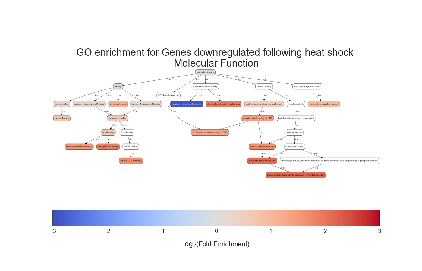
Gene Ontology terms have a somewhat hierarchical relationship that is defined as a directed a-cyclic graph (DAG). This means that each GO term is a node in the graph, and that each node has defined parents that are less specific than itself, going up to the top of the graph.
We can see that in this example the GO term ‘hexose biosynthetic process’ has two parents, one of which is the less specific term ‘hexose metabolic process’, and these relationships go all the way up to the GO term ‘metabolic process’.
Due to the relationships defined between GO terms, when a gene is annotated with a specific GO term, it makes sense that all of the less-specific parents of this GO term will also apply to said gene.
Therefore, when performing GO enrichment, we would usually ‘propagate’ every GO annotation to all of the GO terms upstream to it, all the way to the top of the GO graph.
Unfortunately, propagating GO annotations comes with some issues:
the defined relationship between GO terms introduces dependencies between neighboring GO terms, leading to correlation between enrichment results of different GO terms, and under-estimation of the False Discovery Rate of our analysis.
Moreover, since more specific GO terms by definition have less annotations than their less-specific parents, the most statistically significant enrichment results usually belong to the least-specific GO terms, which are not very biologically relevant.
To deal with this problem, several alternative propagation methods were developed to help de-correlate the GO graph structure and increase the specificity of our results without compromising accuracy.
You can read more about some suggested methods in the following publication:
https://pubmed.ncbi.nlm.nih.gov/16606683/
RNAlysis implements three of these propagation methods: elim, weight, and all.m.
You can decide which propagation method to use by specifying the propagation_method parameter: ‘no’ for no propagation of GO annotations, ‘classic’ for classic propagation of GO annotations, and ‘elim’/’weight’/’all.m’ for propagation using the elim/weight/all.m propagation algorithms.
If you don’t specify which propagation method to use in enrichment analysis, the elim method will be used by default.
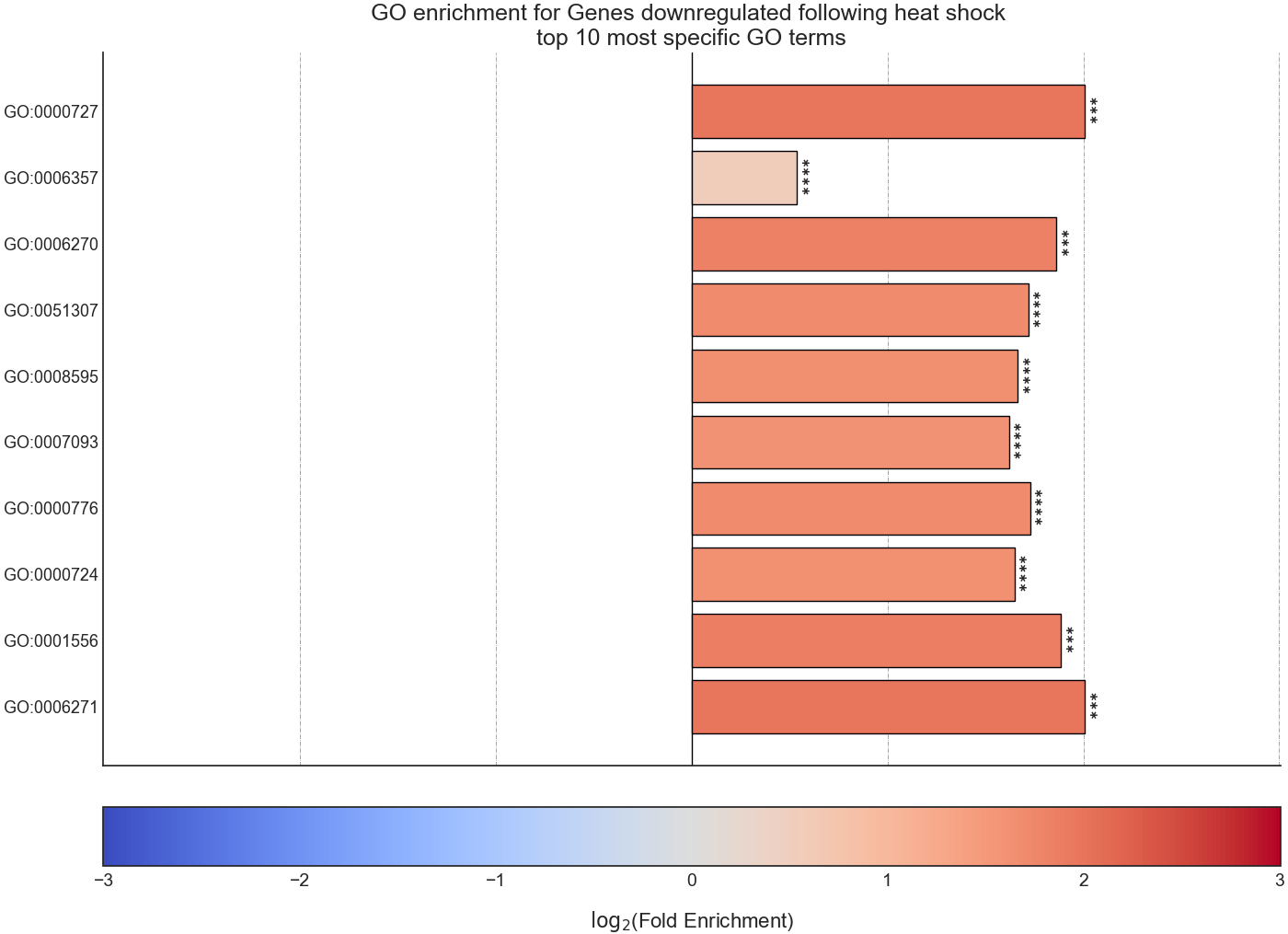
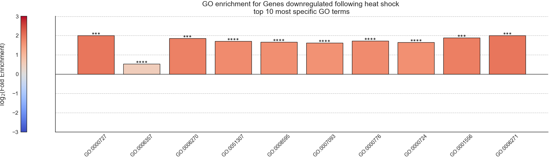
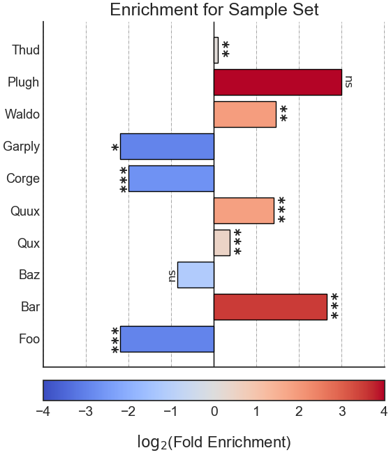
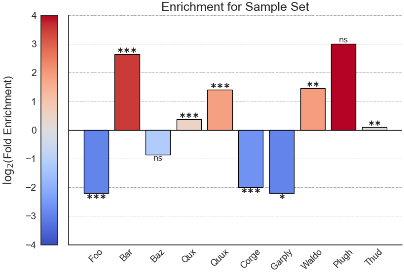
After RNAlysis is done calculating the results of your enrichment analysis, it will automatically plot a summary of the enrichment results.
RNAlysis plots the results as a bar plot, with the Y axis showing log2 fold enrichment, and asterisks indicating whether this enrichment is statistically significant after correcting for multiple comparisons.
You can determine the orientation of the bar plot (horizontal or vertical) using the plot_horizontal parameter:
If you want to further customize this plot, you can request RNAlysis to return a Matplotlib Figure object of the barplot, by using the return_fig parameter.
If you don’t specify plotting parameters, RNAlysis will generate a horizontal bar plot by default, and will not return a Matplotlib Figure object of the bar plot.
In addition, RNAlysis can generate an ontology graph, depicting all of the statistically significant GO terms and their hierarchical relationships:
‘samples’ is the number of features that were used in the enrichment set. ‘obs’ is the observed number of features positive for the attribute in the enrichment set.
‘exp’ is the expected number of features positive for the attribute in the background set. ‘log2_fold_enrichment’ is log2 of the fold change ‘obs’/’exp’.
Define the correct organism and gene ID type for your dataset
Since KEGG annotations refer to specific gene products, which can differ between different species, RNAlysis needs to know which organism your dataset refers to.
The organism can be specified as either the organism’s name, or the organism’s NCBI Taxon ID (for example: 6239 for Caenorhabditis elegans).
It is recommended to manually determine your organism’s NCBI Taxon ID to avoid mischaracterization of annotations.
However, if you are not sure, RNAlysis will attempt to automatically determine the correct organism by default, based on the gene IDs in your FeatureSet.
Furthermore, since different annotations use different gene ID types to annotate the same gene products (such as UniProtKB ID, Entrez Gene ID, or Wormbase WBGene), RNAlysis can translate gene IDs from one gene ID type to another.
In order to do that, you need to specify which gene ID type your dataset uses.
In enrichment analysis, we test whether our set of genomic features is enriched/depleted for a certain KEGG pathway, in comparison to a more generalized set of genomic features that we determined as ‘background’.
This could be the set of all protein-coding genes, the set of all genomic features that show expression above a certain threshold, or any other set of background genes which you deem appropriate. Importantly, the background set must contain all of the genes in the enrichment set.
Enrichment analysis is usually performed on protein-coding genes. Therefore, by default, RNAlysis uses all of the protein-coding genes that have at least one KEGG annotation as a background set.
If you don’t want to use the default setting, there are two methods of defining the background set:
The first method is to specify a biotype (such as ‘protein_coding’, ‘miRNA’ or ‘all’) under the parameter ‘biotype’:
>>> en.kegg_enrichment(biotype='all')
In this example, instead of using all of the protein-coding genes that have GO Annotations as background, we use every genomic feature with GO Annotations as background.
When specifying a biotype, the Biotype Reference Table that you specified is used to determine the biotype of each genomic feature.
The second method of defining the background set is to define a specific set of genomic features to be used as background:
In this example, our background set consists of feature1, feature2 and feature3.
It is not possible to specify both a biotype and a specific background set.
If some of the features in the background set or the enrichment set do no appear in the Reference Table, they will be ignored when calculating enrichment.
Significance testing for KEGG enrichment analysis can be done using either the Hypergeometric Test, Fisher’s Exact Test, or a randomization test.
The hypergeometric test is defined as: Given M genes in the background set, n genes in the test set, with N genes from the background set belonging to a specific attribute (‘success’) and X genes from the test set belonging to that attribute.
If we were to randomly draw n genes from the background set (without replacement), what is the probability of drawing X or more (in case of enrichment)/X or less (in case of depletion) genes belonging to the given attribute?
The Fisher’s Exact test is similar in principle to the hypergeometric test, but is two-tailed by default, as opposed to the hypergeometric test which examines enrichment and depletion separately.
The randomization test is defined as: Given M genes in the background set, n genes in the test set, with N genes from the background set belonging to a specific attribute and X genes from the test set belonging to that attribute.
We performs the number of randomizations specified by the user (10,000 by default).
In each randomization we randomly draw a set of n genes from the background set (without replacement), and marks the randomization as a ‘success’ if the number of genes in the random set belonging to the attribute is >= X (in case of enrichment) or <= X (in case of depletion).
The p-values are calculated as (number of sucesses + 1)/(number of repetitions + 1).
This is a positive-bias estimator of the exact p-value, which avoids exactly-zero p-values.
You can read more about the topic in the following publication: https://www.ncbi.nlm.nih.gov/pubmed/21044043
If you don’t specify which statistical test you want to use, the Fisher’s Exact Test will be used by default.
To choose the statistical test you want to use, utilize the statistical_test parameter, which accepts either ‘fisher’, ‘hypergeometric’, or ‘randomization’.
If you choose to use a randomization test, you can specify the number of randomization repititions to run using the randomization_reps parameter, and set the random seed using the random_seed parameter.
After RNAlysis is done calculating the results of your enrichment analysis, it will automatically plot a summary of the enrichment results.
RNAlysis plots the results as a bar plot, with the Y axis showing log2 fold enrichment, and asterisks indicating whether this enrichment is statistically significant after correcting for multiple comparisons.
You can determine the orientation of the bar plot (horizontal or vertical) using the plot_horizontal parameter:
If you want to further customize this plot, you can request RNAlysis to return a Matplotlib Figure object of the barplot, by using the return_fig parameter.
If you don’t specify plotting parameters, RNAlysis will generate a horizontal bar plot by default, and will not return a Matplotlib Figure object of the bar plot.
‘samples’ is the number of features that were used in the enrichment set. ‘obs’ is the observed number of features positive for the attribute in the enrichment set.
‘exp’ is the expected number of features positive for the attribute in the background set. ‘log2_fold_enrichment’ is log2 of the fold change ‘obs’/’exp’.
Using the enrichment module, you can perform enrichment analysis for user-defined attributes (such as ‘genes expressed in intestine’, ‘epigenetic genes’, ‘genes that have paralogs’). The enrichment analysis can be performed using either the hypergeometric test or a randomization test.
Enrichment analysis for user-defined attributes is performed using FeatureSet.user_defined_enrichment. We will start by creating an FeatureSet object:
Choose which user-defined attributes to calculate enrichment for
Our attributes should be defined in a Reference Table csv file. You can read more about Reference Tables and their format in the section Set and load a Reference Table.
Once we have a Reference Table, we can perform enrichment analysis for those attributes using the function FeatureSet.enrich_randomization.
If your Reference Tables are set to be the default Reference Tables (as explained in Set and load a Reference Table) you do not need to specify them when calling enrich_randomization. Otherwise, you need to specify your Reference Tables’ path.
The names of the attributes you want to calculate enrichment for can be specified as a list of names (for example, [‘attribute1’, ‘attribute2’]).
In enrichment analysis, we test whether our set of genomic features is enriched/depleted for a certain attribute, in comparison to a more generalized set of genomic features that we determined as ‘background’.
This could be the set of all protein-coding genes, the set of all genomic features that show expression above a certain threshold, or any other set of background genes which you deem appropriate. Importantly, the background set must contain all of the genes in the enrichment set.
Enrichment analysis is usually performed on protein-coding genes. Therefore, by default, RNAlysis uses all of the protein-coding genes that appear in the Attribute Reference Table as a background set.
If you don’t want to use the default setting, there are two methods of defining the background set:
The first method is to specify a biotype (such as ‘protein_coding’, ‘miRNA’ or ‘all’) under the parameter ‘biotype’:
In this example, instead of using all of the protein-coding genes in the Attribute Reference Table as background, we use all of the genomic features in the Attribute Reference Table as background.
When specifying a biotype, the Biotype Reference Table that you specified is used to determine the biotype of each genomic feature.
The second method of defining the background set is to define a specific set of genomic features to be used as background:
In this example, our background set consists of feature1, feature2 and feature3.
It is not possible to specify both a biotype and a specific background set.
If some of the features in the background set or the enrichment set do no appear in the Reference Table, they will be ignored when calculating enrichment.
Significance testing for enrichment analysis can be done using either the Hypergeometric Test, Fisher’s Exact Test, or a randomization test.
The hypergeometric test is defined as: Given M genes in the background set, n genes in the test set, with N genes from the background set belonging to a specific attribute (‘success’) and X genes from the test set belonging to that attribute.
If we were to randomly draw n genes from the background set (without replacement), what is the probability of drawing X or more (in case of enrichment)/X or less (in case of depletion) genes belonging to the given attribute?
The Fisher’s Exact test is similar in principle to the hypergeometric test, but is two-tailed by default, as opposed to the hypergeometric test which examines enrichment and depletion separately.
The randomization test is defined as: Given M genes in the background set, n genes in the test set, with N genes from the background set belonging to a specific attribute and X genes from the test set belonging to that attribute.
We performs the number of randomizations specified by the user (10,000 by default).
In each randomization we randomly draw a set of n genes from the background set (without replacement), and marks the randomization as a ‘success’ if the number of genes in the random set belonging to the attribute is >= X (in case of enrichment) or <= X (in case of depletion).
The p-values are calculated as (number of sucesses + 1)/(number of repetitions + 1).
This is a positive-bias estimator of the exact p-value, which avoids exactly-zero p-values.
You can read more about the topic in the following publication: https://www.ncbi.nlm.nih.gov/pubmed/21044043
If you don’t specify which statistical test you want to use, the Fisher’s Exact Test will be used by default.
To choose the statistical test you want to use, utilize the statistical_test parameter, which accepts either ‘fisher’, ‘hypergeometric’, or ‘randomization’.
If you choose to use a randomization test, you may specify the number of randomization repititions to run using the randomization_reps parameter, and set the random seed using the random_seed parameter.
After performing enrichment analysis, RNAlysis will automatically plot a summary of your enrichment results as a bar plot of log-transformed enrichment scores.
You can determine the orientation of the bar plot (horizontal or vertical) using the plot_horizontal parameter:
If you want to further customize your plot, you can retreive the matplotlib Figure object of your plot using the return_fig parameter.
When it is set as ‘True’, RNAlysis will return the Figure object it generated in addition to the results table.
Running enrichment analysis will calculate enrichment for each of the specified attributes, and return a pandas DataFrame in the following format:
samples
obs
exp
log2_fold_enrichment
pval
padj
significant
attribute1
1327
451
319.52
0.49722119558
0.0000999
0.0000999
True
attribute2
1327
89
244.87
-1.46013879322
0.0000999
0.0000999
True
‘samples’ is the number of features that were used in the enrichment set. ‘obs’ is the observed number of features positive for the attribute in the enrichment set.
‘exp’ is the expected number of features positive for the attribute in the background set. ‘log2_fold_enrichment’ is log2 of the fold change ‘obs’/’exp’.
Performing enrichment analysis for non-categorical user-defined attributes
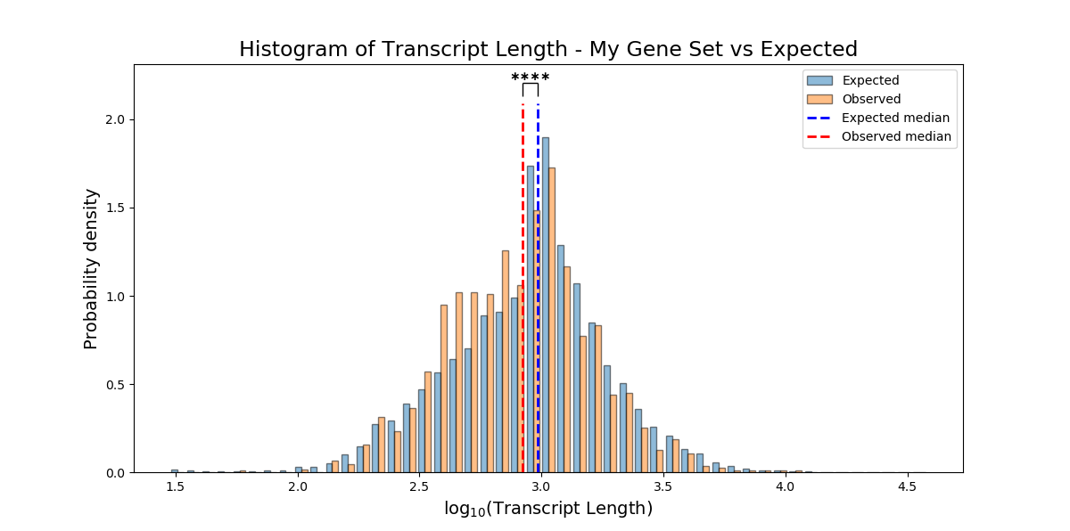
Instead of peforming enrichment analysis for categorical attributes (“genes which are expressed exclusively in neurons”, “genes enriched in males”, “epigenetic gene-products”, etc), you can test whether your FeatureSet is enriched for a non-categorical attribute (“number of paralogs”, “gene length”, or any other numeric attribute) using the function FeatureSet.non_categorical_enrichment().
Choose which user-defined non-categorical attributes to calculate enrichment for
The attributes should be defined in an Attribute Reference Table csv file. You can read more about Reference Tables and their format in the section Set and load a Reference Table.
Once we have an Attirubte Reference Table, we can perform enrichment analysis for those non-categorical attributes using the function FeatureSet.non_categorical_enrichment.
If your Reference Tables are set to be the default Reference Tables (as explained in Set and load a Reference Table) you do not need to specify them when calling non_categorical_enrichment. Otherwise, you need to specify your Reference Tables’ path.
The names of the attributes you want to calculate enrichment for can be specified as a list of names (for example, [‘attribute1’, ‘attribute2’]).
Note that the variables you use for non-categorical enrichment analysis must be non-categorical, and must be defined for every genomic feature in the background and test sets (meaning, no NaN values).
In enrichment analysis, we test whether our set of genomic features is enriched/depleted for a certain attribute, in comparison to a more generalized set of genomic features that we determined as ‘background’.
This could be the set of all protein-coding genes, the set of all genomic features that show expression above a certain threshold, or any other set of background genes which you deem appropriate. Importantly, the background set must contain all of the genes in the enrichment set.
Enrichment analysis is usually performed on protein-coding genes. Therefore, by default, RNAlysis uses all of the protein-coding genes that appear in the Attribute Reference Table as a background set.
If you don’t want to use the default setting, there are two methods of defining the background set:
The first method is to specify a biotype (such as ‘protein_coding’, ‘miRNA’ or ‘all’) under the parameter ‘biotype’:
In this example, instead of using all of the protein-coding genes in the Attribute Reference Table as background, we use all of the genomic features in the Attribute Reference Table as background.
When specifying a biotype, the Biotype Reference Table that you specified is used to determine the biotype of each genomic feature.
The second method of defining the background set is to define a specific set of genomic features to be used as background:
In this example, our background set consists of feature1, feature2 and feature3.
It is not possible to specify both a biotype and a specific background set.
If some of the features in the background set or the enrichment set do no appear in the Reference Table, they will be ignored when calculating enrichment.
When calculating enrichment for a non-categorical attribute, you can use either a parametric or non-parametric statistical test.
If the parametric_test parameter is True, RNAlysis will calculate enrichment using the one-sample Student’s T-test, comparing the value of the non-categorical attribute in your enrichment set to the mean value of the non-categorical attribute in the background set.
If the parametric_test parameter is False, RNAlysis will calculate enrichment using the non-parametric one-sample Sign test, comparing the value of the non-categorical attribute in your enrichment set to the median value of the non-categorical attribute in the background set.
The parametric T-test assumes that the values of your non-categorical attribute distribute normally. Therefore, if you are not sure your data meets this assumption, it is recommended to use the less-powerful non-parametric test.
If you don’t specify the statistical test, RNAlysis will automatically use a non-parametric test.
The results of non-categorical enrichment analysis will be plotted as a histogram, comparing the distribution of the non-categorical attribute within the enrichment set compared to the background set.
If you used a parametric test, the mean of each set will be marked on the histogram. Alternatively, if you used a non-parametric test, the median of each set will be marked on the graph.
The enrichment results of each attribute will be plotted in a different Figure.
To better fit the visualization of the results to your needs, you can specify two parameters:
plot_log_scale can accept either True or False, and will determine whether the X-axis of the histogram will be plotting on a logarithmic or linear scale.
`plot_style’ can accept either ‘overlap’ or ‘interleaved’, and will draw the histogram in one of the following two styles:
If you don’t specify plotting parameters, RNAlysis will plot the histogram on a logarithmic scale using the ‘overlap’ style by default.
If you want to further customize your plot, you can retreive the matplotlib Figure object of your plot using the return_fig parameter.
When it is set as ‘True’, RNAlysis will return the Figure object it generated in addition to the results table.
Running non-categorical enrichment analysis will calculate enrichment for each of the specified attributes, and return a pandas DataFrame in the following format:
samples
obs
exp
pval
padj
significant
attribute1
1327
451
319.52
0.0000999
0.0000999
True
attribute2
1327
89
244.87
0.0000999
0.0000999
True
‘samples’ is the number of features that were used in the enrichment set. ‘obs’ is the observed mean/median (depending if the statistical test was parametric or not) value of the non-categorical attribute in the enrichment set.
‘exp’ is the expected mean/median value of the non-categorical attribute in the background set.
Performing set operations and visualisation on multiple FeatureSet objects
Similarly to Filter objects, it is possible to use set operations such as union, intersection, difference and symmetric difference to combine the feature sets of multiple FeatureSet objects. Those set operations can be applied to both FeatureSet objects and python sets. The objects don’t have to be of the same subtype - you can, for example, look at the union of an FeatureSet object and a python set:
When performing set operations, the return type will always be a python set. This means you can use the output of the set operation as an input for yet another set operation, or as input to a new FeatureSet object.
In addition, the enrichment module includes functions for visualisation of sets and overlap, such as enrichment.venn_diagram() and enrichment.upset_plot().
Both functions receive a similar input: a dictionary whose keys are the names of the sets, and values are either FeatureSet objects, Filter objects, sets of genomic feature names, or the name of an attribute from the Attribute Reference Table (you can read more about attributes in Set and load a Reference Table).
Venn diagrams are limited to 2-3 sets:
It is possible to save the feature indices from an FeatureSet object to a .txt file, for use in online enrichment tools or simply to share the list of genomic features. This is done with the ‘save_txt’ function:
>>> en.save_txt('D:\path\filename')
The feature indices will be saved to the text file in the specified path, separated by newline (’n’).
The RankedSet class represents a set of genomic features which are ranked by an inherent order. For example, genes could be ranked based on their mean expression level, their fold change between a pair of conditions, etc.
RankedSet objects behave similarly to FeatureSet objects, but in addition they support single-set enrichment analysis - enrichment analysis without a background set.
The statistical test used to test significance in single-set enrichment analysis is the generalized minimum hypergeometric test (XL-mHG), which measures the enrichment of the genomic features at the top and bottom of your ranked gene set compared to the rest of the gene set.
You can read more about the minimum hypergeometric test and its generalized version the XL-mHG test in the following publications:
https://journals.plos.org/ploscompbiol/article?id=10.1371/journal.pcbi.0030039https://arxiv.org/abs/1507.07905
RankedSet objects can be initialized by one of two methods.
The first method is to specify an existing Filter object:
>>> my_filter_obj=filtering.CountFilter('tests/test_files/counted.csv')# create a Filter object>>> my_ranked_set=enrichment.RankedSet(my_filter_obj,'a name for my set')
When using this method, the ranking of the genomic features will be determined by their current order within the Filter object. You can use the ‘sort’ method of your Filter object to modify the current order of genomic features within the Filter object.
The second method is to directly specify a list, tuple, or numpy array of genomic feature names:
>>> my_list=['WBGene00000001','WBGene0245200',' WBGene00402029']>>> my_ranked_set=enrichment.RankedSet(my_list,'a name for my set')
RankedSet objects have three attributes: ranked_genes, a numpy array containing the ranked genomic features; gene_set, a python set containing the genomic features; and set_name, a string that describes the feature set (optional).
Performing single-set GO Enrichment analysis without a background set
Single-set GO Enrichment works much the same as normal Go Enrichment analysis, with two key differences:
First, when performing single-set GO Enrichment you do not define a background set to comapre your enrichment gene set against. Instead, you supply a RankedSet that defines a meaningful ranking for your gene set.
Second, you cannot specify which statistical test to use, since the XL-mHG test has to be used.
An example for running single-set GO Enrichment would look like so:
Performing single-set KEGG Enrichment analysis without a background set
Single-set KEGG Enrichment works much the same as normal KEGG Enrichment analysis, with two key differences:
First, when performing single-set KEGG Enrichment you do not define a background set to comapre your enrichment gene set against. Instead, you supply a RankedSet that defines a meaningful ranking for your gene set.
Second, you cannot specify which statistical test to use, since the XL-mHG test has to be used.
An example for running single-set KEGG Enrichment would look like so:
Performing single-set enrichment analysis for user-defined attributes without a background set
Single-set enrichment analysis for user-defined attributes works much the same as normal enrichment analysis, with two key differences:
First, when performing single-set enrichment you do not define a background set to comapre your enrichment gene set against. Instead, you supply a RankedSet that defines a meaningful ranking for your gene set.
Second, you cannot specify which statistical test to use, since the XL-mHG test has to be used.
An example for running single-set enrichment analysis would look like so:
If you want to plot existing enrichment results using RNAlysis, you can use the enrichment.plot_enrichment_results() function. It employs a similar API to the enrichment functions in the enrichment modules, but accepts pre-calculated DataFrames.
To visualize set intersection using a Venn Diagram or UpSet plot, you first need to define the sets you want to visualize.
Those sets can be represented using a python dictionary, where each key represents the name of the set, and the corresponding value represents the set’s content (the genomic features that are part of the set).
There are three ways of specifying a set’s content:
A python set containing the names of the genomic features
A FeatureSet or RankedSet object containing the names of the genomic features
After defining the dictionary of sets, we can use it to plot set intersection via the enrichment.venn_diagram() or enrichment.upset_plot() functions.
Venn diagrams in RNAlysis are plotted with relatively accurate proportions and overlaps, and therefore only support up to 3 sets.
RNAlysis’s general module (rnalysis.general) contains general functions that can be useful during analysis of RNA sequencing data, including regular expression parsers and setting the Reference Table path.
You can perform enrichment analysis or filtering operations based on user-defined attributes (such as ‘genes expressed in intestine’, ‘epigenetic genes’, ‘genes that have paralogs’).
User-defined attributes should be defined in an Attribute Reference Table csv file. The format of the Attribute Reference Table is one row for each gene/genomic feature, and one column for each attribute. Features that are negative for the attribute (for example, genes that have no paralogs under the attribute ‘genes that have paralogs’) should have the value NaN specified for the attribute, and features that are positive for the attribute (for example, genes that have paralogs under the attribute ‘genes that have paralogs’) should have any value other than NaN. The value could be either a boolean value (in our example, ‘True’ or ‘1’ for genes that have paralogs), a number (in our example, the number of paralogs the gene has or the genomic distance to the nearest paralog), or any other value which is not NaN. See example for an Attribute Reference Table below:
You can perform filtering operations or generate background-sets for enrichment analysis based on user-annotated biotypes (such as ‘protein_coding’, ‘pseudogene’, ‘piRNA’, etc).
User-annotated biotypes should be defined in a Biotype Reference Table csv file. The format of the Biotype Reference Table is one row for each gene/genomic feature, and a column titled ‘biotype’ (case insensitive). See example for a Biotype Reference Table below:
Once we have an Attribute and/or Biotype Reference Table, we can set it to be the default reference table for all future uses of RNAlysis:
>>> from*RNAlysis*importgeneral>>> path="the_new_attribute_reference_table_path">>> general.set_attr_ref_table_path(path)Attribute Reference Table path set as: the_new_attribute_reference_table_path>>> path="the_new_biotype_reference_table_path">>> general.set_biotype_ref_table_path(path)Attribute Reference Table path set as: the_new_biotype_reference_table_path
This will create a file called ‘settings.yaml’, which will store the full paths of your reference tables.
Whenever RNAlysis needs to use an Attribute/Biotype Reference Table and no other path is specified, RNAlysis will automatically use the path saved in the settings file.
The saved path can be changed any time using the general.set_attr_ref_table_path() and general.set_biotype_ref_table_path() functions.
If an Attribute Reference Table path was not previously defined, you will be requested to define it when you run this function.
Parse C. elegans gene names, WBGene indices and sequence names using regular expressions
The general module includes functions which can parse C. elegans gene names (like daf-2 or lin-15B), WBGene indices (like WBGene00023495) and sequence names (like Y55D5A.5 or T23G5.6).
For example, we could extract all WBGene indices from the following string:
>>> from*RNAlysis*importgeneral>>> my_string='''WBGene00000001 and WBGene00000002WBGene00000003 WBGene00000004g '''>>> general.parse_wbgene_string(my_string){'WBGene00000001','WBGene000000002','WBGene00000003','WBGene00000004'}